using OrdinaryDiffEq
using ComponentArrays
using SimpleUnPack
using Plots
Plots.default(linewidth=2)Fig 6.19
Sine wave response of g-protein signalling pathway
_l619(p, t) = p.lt + (p.lt / p.l_AMP) * cospi(2t / p.l_per)

function model619!(D, u, p, t)
    @unpack kRL, kRLm, kGa, kGd0, kG1, Rtotal, Gtotal, lt, l_per, l_AMP = p
    @unpack RL, Ga, Gd = u
    R = Rtotal - RL
    G = Gtotal - Ga - Gd
    Gbg = Ga + Gd
    L = _l619(p, t)
    v1 = kRL * R * L - kRLm * RL
    v2 = kGa * G * RL
    v3 = kGd0 * Ga
    v4 = kG1 * Gd * Gbg
    D.RL = v1
    D.Ga = v2 - v3
    D.Gd = v3 - v4
    nothing
end
model619! (generic function with 1 method)ps619 = ComponentArray(
kRL = 2e6,
kRLm = 0.01,
kGa = 1e-5,
kGd0 = 0.11,
kG1 = 1.0,
Rtotal = 4e3,
Gtotal = 1e4,
lt = 1e-9,
l_per = 200.0,
l_AMP = 5.0
)
ics619 = ComponentArray(
RL = 0.0,
Ga = 0.0,
Gd = 0.0,
)
tend = 1000.0
prob619 = ODEProblem(model619!, ics619, (0.0, tend), ps619)ODEProblem with uType ComponentArrays.ComponentVector{Float64, Vector{Float64}, Tuple{ComponentArrays.Axis{(RL = 1, Ga = 2, Gd = 3)}}} and tType Float64. In-place: true Non-trivial mass matrix: false timespan: (0.0, 1000.0) u0: ComponentVector{Float64}(RL = 0.0, Ga = 0.0, Gd = 0.0)
@time sol619 = solve(prob619, Tsit5())
pl1 = plot(t-> sol619(t).Ga, 0.0, tend, label="Ga", xlabel="Time", ylabel="Concentration", title="Fig 6.19 A")

pl2 = plot(t -> _l619(ps619, t) * 1E9, 0.0, tend, label="L", xlabel="Time", ylabel="Concentration (nM)", title="Fig 6.19 B")

plot(pl1, pl2, layout=(2,1))
2.085610 seconds (10.89 M allocations: 524.891 MiB, 2.50% gc time, 93.93% compilation time)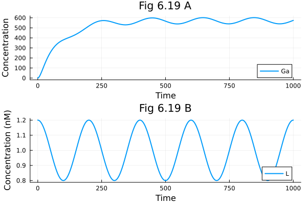
This notebook was generated using Literate.jl.
Back to top