using OrdinaryDiffEq
using ComponentArrays
using SimpleUnPack
using Plots
Plots.default(linewidth=2)Fig 3.03
Michaelis-Menten kinetics
Enzyme kinetics full model
_e303(u, p, t) = p.ET - u.ES
function model303!(du, u, p, t)
    @unpack k1, km1, k2 = p
    @unpack S, ES, P = u
    E = _e303(u, p, t)
    v1 = k1 * S * E - km1 * ES
    v2 = k2 * ES
    du.S = -v1
    du.ES = v1 - v2
    du.P = v2
    nothing
end
model303! (generic function with 1 method)ps303 = ComponentArray(
k1 = 30.0,
km1 = 1.0,
k2 = 10.0,
ET = 1.0
)
u0 = ComponentArray(
S = 5.0,
ES = 0.0,
P = 0.0
)
tend = 1.0
prob303 = ODEProblem(model303!, u0, tend, ps303)ODEProblem with uType ComponentArrays.ComponentVector{Float64, Vector{Float64}, Tuple{ComponentArrays.Axis{(S = 1, ES = 2, P = 3)}}} and tType Float64. In-place: true Non-trivial mass matrix: false timespan: (0.0, 1.0) u0: ComponentVector{Float64}(S = 5.0, ES = 0.0, P = 0.0)
@time sol = solve(prob303) 11.947457 seconds (38.33 M allocations: 1.879 GiB, 2.38% gc time, 100.00% compilation time)retcode: Success
Interpolation: 3rd order Hermite
t: 40-element Vector{Float64}:
0.0
6.665333466693315e-6
7.331866813362645e-5
0.000486426499836535
0.0012463104267083492
0.0022559163259547044
0.003638919897606555
0.005455833654299618
0.007824959148420711
0.010840766457437317
⋮
0.6498572831449281
0.6992361771444529
0.7455747547375974
0.7903699863468574
0.8349926420141908
0.8806910765547713
0.9286579911037935
0.9801092501915283
1.0
u: 40-element Vector{ComponentArrays.ComponentVector{Float64, Vector{Float64}, Tuple{ComponentArrays.Axis{(S = 1, ES = 2, P = 3)}}}}:
ComponentVector{Float64}(S = 5.0, ES = 0.0, P = 0.0)
ComponentVector{Float64}(S = 4.999000802751873, ES = 0.000999163942258781, P = 3.330586857606668e-8)
ComponentVector{Float64}(S = 4.989074749914229, ES = 0.010921237104096317, P = 4.0129816751718436e-6)
ComponentVector{Float64}(S = 4.930127945660642, ES = 0.06969993841061332, P = 0.00017211592874508686)
ComponentVector{Float64}(S = 4.832226260206192, ES = 0.16669487186074256, P = 0.0010788679330659236)
ComponentVector{Float64}(S = 4.720095602191208, ES = 0.27657130144488123, P = 0.0033330963639114255)
ComponentVector{Float64}(S = 4.593086950718923, ES = 0.3988758764938655, P = 0.008037172787212131)
ComponentVector{Float64}(S = 4.461543546979021, ES = 0.5219980795240163, P = 0.016458373496963406)
ComponentVector{Float64}(S = 4.332646087873498, ES = 0.6370812621468814, P = 0.03027264997962138)
ComponentVector{Float64}(S = 4.214625749264197, ES = 0.7343117806650907, P = 0.051062470070712705)
⋮
ComponentVector{Float64}(S = 0.04626411606378614, ES = 0.2691867228327527, P = 4.684549161103462)
ComponentVector{Float64}(S = 0.020977105513513086, ES = 0.1835757278582751, P = 4.795447166628213)
ComponentVector{Float64}(S = 0.010414950263948735, ES = 0.12369155788070173, P = 4.865893491855351)
ComponentVector{Float64}(S = 0.00565646792272255, ES = 0.08276248765840352, P = 4.911581044418876)
ComponentVector{Float64}(S = 0.0032796739340834164, ES = 0.05484216590159223, P = 4.941878160164326)
ComponentVector{Float64}(S = 0.0019694258218005234, ES = 0.035753678406086016, P = 4.962276895772115)
ComponentVector{Float64}(S = 0.0011916706791066725, ES = 0.02273524960318758, P = 4.9760730797177075)
ComponentVector{Float64}(S = 0.0007101807195001165, ES = 0.013958539864174141, P = 4.985331279416328)
ComponentVector{Float64}(S = 0.0005834152171657496, ES = 0.011555343089102596, P = 4.987861241693734)
pl303 = plot(sol, xlabel="Time (AU)", ylabel="Concentration (AU)", legend=:right, title="Fig 3.03", labels=["S (full)" "ES (full)" "P (full)"])

let ts = 0:0.01:tend
    es = (t) -> _e303(sol(t), ps303, t)
    plot!(pl303, ts, es, label="E (full)")
end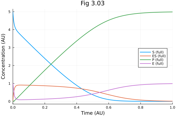
QSSA of ES complex
_s303mm(u, p, t) = p.S0 - u.P
function model303mm!(du, u, p, t)
    @unpack k1, km1, k2, ET = p
    @unpack P = u
    S = _s303mm(u, p, t)
    ES = (k1 * S * ET) / (km1 + k2 + k1 * S)
    v2 = k2 * ES
    du.P = v2
    nothing
end

ps303mm = ComponentArray(ps303; S0=5.0)
prob303mm = ODEProblem(model303mm!, ComponentArray(P=0.0), tend, ps303mm)
ODEProblem with uType ComponentArrays.ComponentVector{Float64, Vector{Float64}, Tuple{ComponentArrays.Axis{(P = 1,)}}} and tType Float64. In-place: true Non-trivial mass matrix: false timespan: (0.0, 1.0) u0: ComponentVector{Float64}(P = 0.0)
@time sol303mm = solve(prob303mm) 11.739110 seconds (38.13 M allocations: 1.872 GiB, 2.05% gc time, 100.00% compilation time)retcode: Success
Interpolation: 3rd order Hermite
t: 14-element Vector{Float64}:
0.0
9.999999999999999e-5
0.0010999999999999998
0.011099999999999997
0.0782815192255917
0.22560725880659876
0.40777510082471
0.5814448248891889
0.6444132780246575
0.709328257260174
0.7626632358601979
0.8371444047425067
0.9162616372026308
1.0
u: 14-element Vector{ComponentArrays.ComponentVector{Float64, Vector{Float64}, Tuple{ComponentArrays.Axis{(P = 1,)}}}}:
ComponentVector{Float64}(P = 0.0)
ComponentVector{Float64}(P = 0.0009316710873866917)
ComponentVector{Float64}(P = 0.010247728722854758)
ComponentVector{Float64}(P = 0.10334216159542618)
ComponentVector{Float64}(P = 0.7253458014622206)
ComponentVector{Float64}(P = 2.061211027540912)
ComponentVector{Float64}(P = 3.6086931554952244)
ComponentVector{Float64}(P = 4.7352540338477445)
ComponentVector{Float64}(P = 4.921045864324829)
ComponentVector{Float64}(P = 4.982819834816748)
ComponentVector{Float64}(P = 4.995791653645537)
ComponentVector{Float64}(P = 4.999292966351351)
ComponentVector{Float64}(P = 4.9998890349369844)
ComponentVector{Float64}(P = 4.999982400534711)
ts = 0:0.01:tend0.0:0.01:1.0let ts = 0:0.01:tend
ss = sol(ts, idxs=1).u
pp = sol(ts, idxs=3).u
ss_mm = _s303mm.(sol303mm(ts).u, Ref(ps303mm), ts)
pp_mm = sol303mm(ts, idxs=1).u
fig = plot(ts, [ss pp], label=["S (full)" "P (full)"], line=(:dash))
plot!(fig, ts, [ss_mm pp_mm], label=["S (MM)" "P (MM)"])
plot!(fig, title="Fig. 3.03",
xlabel="Time (AU)", ylabel="Concentration (AU)",
xlims=(0., tend), ylims=(0., 5.), legend=:right)
fig
end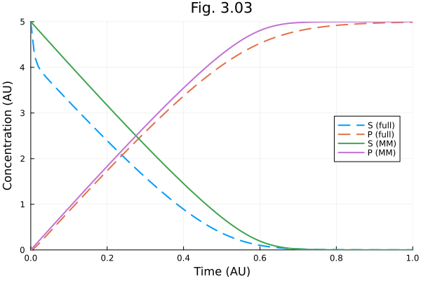
This notebook was generated using Literate.jl.