using Plots
using DataInterpolations: LinearInterpolation
using StatsBase: Weights, sample
using Statistics: mean
using Random
using DisplayAs: PNG    ## For faster rendering
Random.seed!(2024)Random.TaskLocalRNG()using Plots
using DataInterpolations: LinearInterpolation
using StatsBase: Weights, sample
using Statistics: mean
using Random
using DisplayAs: PNG ## For faster rendering
Random.seed!(2024)Random.TaskLocalRNG()Stochastic chemical reaction: Gillespie Algorithm (direct and first reaction method) Adapted from: Chemical and Biomedical Engineering Calculations Using Python Ch.4-3
function ssa_alg(model, u0::AbstractVector, tend, p, stoich; tstart=zero(tend), method=:direct)
    t = tstart   ## Current time
    ts = [t]     ## Time points
    u = copy(u0) ## Current state
    us = copy(u') ## States over time
    while t < tend
        a = model(u, p, t)               ## propensities
        if method == :direct
            dt = randexp() / sum(a)          ## Time step for the direct method
            du = sample(stoich, Weights(a))  ## Choose the stoichiometry for the next reaction
        elseif method == :first
            dts = randexp(length(a)) ./ a   ## time scales of all reactions
            i = argmin(dts)                 ## Choose the most recent reaction to occur
            dt = dts[i]
            du = stoich[i]
        else
            error("Method should be either :direct or :first")
        end
        u .+= du   ## Update time
        t += dt    ## Update time
        us = [us; u']  ## Append state
        push!(ts, t)   ## Append time point
    end
    return (t=ts, u=us)
end
ssa_alg (generic function with 1 method)Propensity model for this example reaction. Reaction of A <-> B with rate constants k1 & k2
model(u, p, t) = [p.k1 * u[1], p.k2 * u[2]]model (generic function with 1 method)parameters = (k1=1.0, k2=0.5)(k1 = 1.0, k2 = 0.5)Stoichiometry for each reaction
stoich = [[-1, 1], [1, -1]]2-element Vector{Vector{Int64}}:
[-1, 1]
[1, -1]Initial conditions (Usually discrete values)
u0 = [200, 0]2-element Vector{Int64}:
200
0Simulation time
tend = 10.010.0Solve the problem using both direct and first reaction method
@time soldirect = ssa_alg(model, u0, tend, parameters, stoich; method=:direct)
@time solfirst = ssa_alg(model, u0, tend, parameters, stoich; method=:first)
0.685222 seconds (928.30 k allocations: 60.691 MiB, 19.67% gc time, 99.51% compilation time)
0.005784 seconds (16.35 k allocations: 14.937 MiB)(t = [0.0, 0.006874672879606227, 0.0070050915014185, 0.01329115182676454, 0.015335530116774018, 0.01942319769041779, 0.021346508038833215, 0.02345030020299408, 0.025497753122539372, 0.02734483697039726 … 9.937773197389458, 9.938360255993572, 9.964450740930666, 9.96564917153764, 9.975440668199402, 9.978594329657025, 9.982318425245289, 9.987213207313044, 9.995833233887383, 10.024199143896238], u = [200 0; 199 1; … ; 75 125; 74 126])Plot the solution from the direct method
plot(soldirect.t, soldirect.u,
    xlabel="time", ylabel="# of molecules",
    title="SSA (direct method)", label=["A" "B"]) |> PNG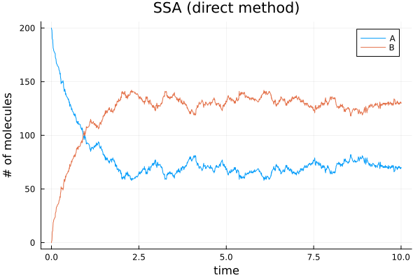
Plot the solution by the first reaction method
plot(solfirst.t, solfirst.u,
    xlabel="time", ylabel="# of molecules",
    title="SSA (1st reaction method)", label=["A" "B"]) |> PNG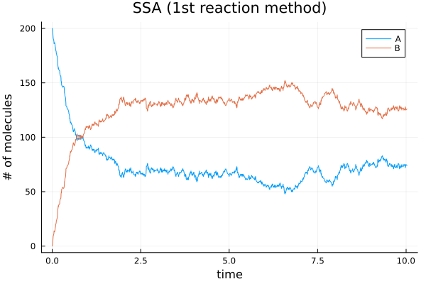
Running 50 simulations
numRuns = 50

@time sols = map(1:numRuns) do _
    ssa_alg(model, u0, tend, parameters, stoich; method=:direct)
end;
0.181422 seconds (760.47 k allocations: 752.427 MiB, 24.61% gc time, 40.07% compilation time)Average values and interpolation
ts = range(0, tend, 101)
a_interp = [LinearInterpolation(sol.u[:, 1], sol.t; cache_parameters=true) for sol in sols]
b_interp = [LinearInterpolation(sol.u[:, 2], sol.t; cache_parameters=true) for sol in sols]
a_avg(t) = mean(i-> i(t), a_interp)
b_avg(t) = mean(i-> i(t), b_interp)
b_avg (generic function with 1 method)Plot the solution
fig1 = plot(xlabel="Time", ylabel="# of molecules", title="SSA (first method) ensemble")

for sol in sols
    plot!(fig1, sol.t, sol.u, linecolor=[:blue :red], linealpha=0.05, label=false)
end

fig1 |> PNG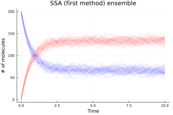
Plot averages
plot!(fig1, a_avg, 0.0, tend, linecolor=:black, linewidth=3, linestyle=:solid, label="Average [A]") |> PNG
plot!(fig1, b_avg, 0.0, tend, linecolor=:black, linewidth=3, linestyle=:dash, label="Average [B]") |> PNG
fig1 |> PNG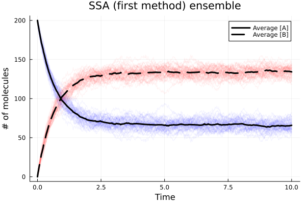
This notebook was generated using Literate.jl.