Plotting with Julia

• JuliaPlots/Plots.jl : powerful and convenient visualization with multiple backends. See also Plots.jl docs

• JuliaPy/PythonPlot.jl : matplotlib in Julia. See also matplotlib docs

• MakieOrg/Makie.jl : a data visualization ecosystem for the Julia programming language, with high performance and extensibility. See also Makie.jl docs

using Plots

Prepare data then plot

f(x) = sin(sin(x) + 1)
xs = 0.0:0.1:4pi
ys = f.(xs)

plot(xs, ys)

Line plots connect the data points

plot(xs, ys)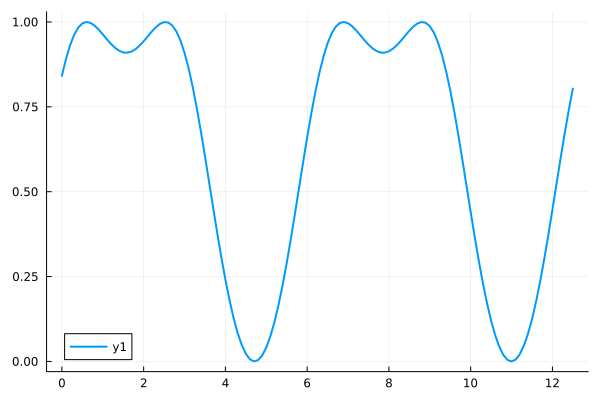

Scatter plots show the data points only

scatter(xs, ys)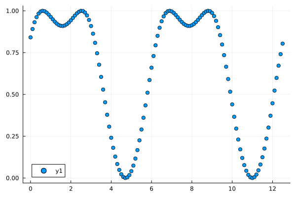

you can trace functions directly

plot(f, xs)

Trace a function within a range

plot(f, 0.0, 4pi)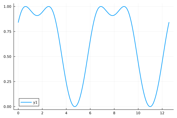

Customization example

plot(f, xs,
    label="My line", legend=:bottom,
    title="My Title",  line=(:red, 3),
    xlim = (0.0, 5.0), ylim = (-1.0, 1.5),
    xlabel="Time", ylabel="My Mood", border=:box)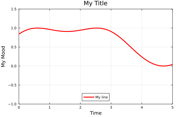

Multiple series: each row is one observation; each column is a variable.

f2(x) = cos(cos(x) + 1)
y2 = f2.(xs)
plot(xs, [ys y2])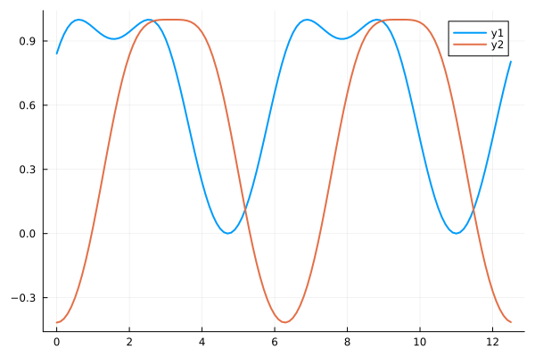

Plotting two functions with customizations

plot(xs, [f, f2], label=["f1" "f2"], linecolor=[:black :green], title="Two time series")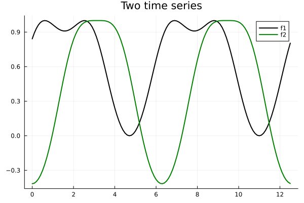

Building the plot in multiple steps in the object-oriented way

xMin = 0.0
xMax = 4.0π
fig = plot(f, xMin, xMax, label="f1", lc=:black)
plot!(fig , f2, xMin, xMax, label="f2", lc=:lightsalmon)
plot!(fig, title = "My title", legend=:outertop)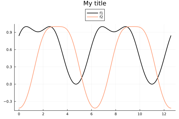

Parametric plot

xₜ(t) = sin(t)
yₜ(t) = sin(2t)

plot(xₜ, yₜ, 0, 2π, leg=false, fill=(0,:orange))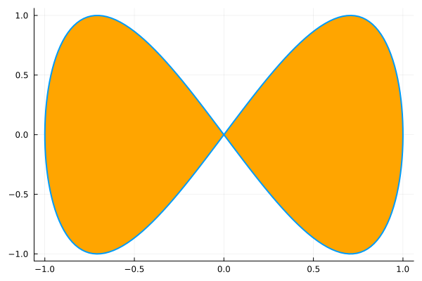

Subplots

ax1 = plot(f, xs)
ax2 = plot(f2, xs)
plot(ax1, ax2)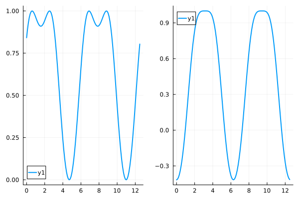

Subplot layout

fig = plot(ax1, ax2, layout=(2, 1))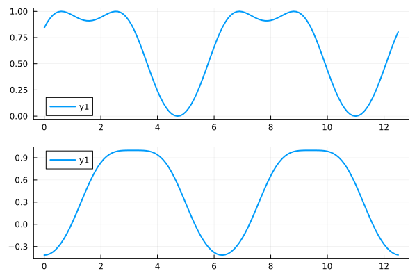

Vector field

Plots.jl

# Quiver plot
quiver(vec(x2d), vec(y2d), quiver=(vec(vx2d), vec(vy2d))

# Or if you have a gradient function ∇f(x,y) -> (vx, vy)
quiver(x2d, y2d, quiver=∇f)

PythonPlot.jl:

using PythonPlot as plt
plt.quiver(X2d, Y2d, U2d, V2d)

See also: matplotlib: quiver plot

using Plots

∇ = \nabla <TAB>

function ∇f(x, y; scale=(x^2 + y^2)^0.25 * 3)
    return [-y, x] ./ scale
end

∇f (generic function with 1 method)

x and y grid points

r = -1.0:0.2:1.0
xx = [x for y in r, x in r]
yy = [y for y in r, x in r]

11×11 Matrix{Float64}:
 -1.0  -1.0  -1.0  -1.0  -1.0  -1.0  -1.0  -1.0  -1.0  -1.0  -1.0
 -0.8  -0.8  -0.8  -0.8  -0.8  -0.8  -0.8  -0.8  -0.8  -0.8  -0.8
 -0.6  -0.6  -0.6  -0.6  -0.6  -0.6  -0.6  -0.6  -0.6  -0.6  -0.6
 -0.4  -0.4  -0.4  -0.4  -0.4  -0.4  -0.4  -0.4  -0.4  -0.4  -0.4
 -0.2  -0.2  -0.2  -0.2  -0.2  -0.2  -0.2  -0.2  -0.2  -0.2  -0.2
  0.0   0.0   0.0   0.0   0.0   0.0   0.0   0.0   0.0   0.0   0.0
  0.2   0.2   0.2   0.2   0.2   0.2   0.2   0.2   0.2   0.2   0.2
  0.4   0.4   0.4   0.4   0.4   0.4   0.4   0.4   0.4   0.4   0.4
  0.6   0.6   0.6   0.6   0.6   0.6   0.6   0.6   0.6   0.6   0.6
  0.8   0.8   0.8   0.8   0.8   0.8   0.8   0.8   0.8   0.8   0.8
  1.0   1.0   1.0   1.0   1.0   1.0   1.0   1.0   1.0   1.0   1.0

Vector fields

quiver(xx, yy, quiver=∇f, aspect_ratio=:equal, line=(:black), arrow=(:closed))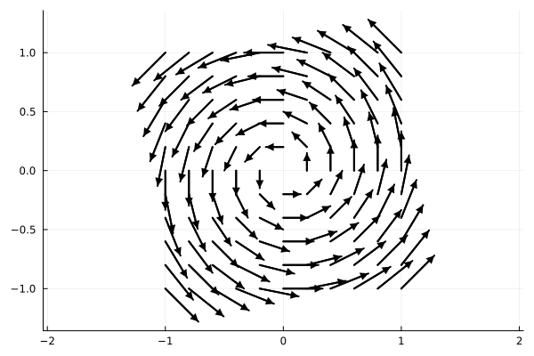

Save figure

savefig([fig_obj,] filename)

Save the current figure

savefig("vector-field.png")

"/home/github/actions-runner-1/_work/mmsb-bebi-5009/mmsb-bebi-5009/.cache/docs/vector-field.png"

Save the figure fig

savefig(fig, "subplots.png")

"/home/github/actions-runner-1/_work/mmsb-bebi-5009/mmsb-bebi-5009/.cache/docs/subplots.png"

---

This notebook was generated using Literate.jl.