Fig 1.09

Hodgkin-Huxley model

using OrdinaryDiffEq
using ModelingToolkit
using Plots
Plots.default(linewidth=2)

Convenience functions

hil(x, k) = x / (x + k)
hil(x, k, n) = hil(x^n, k^n)
exprel(x) = x / expm1(x)

exprel (generic function with 1 method)

HH Neuron model

function build_hh(;name)
    @independent_variables t
    @parameters begin
        E_N = 55.0       ## Reversal potential of Na (mV)
        E_K = -72.0      ## Reversal potential of K (mV)
        E_LEAK = -49.0   ## Reversal potential of leaky channels (mV)
        G_N_BAR = 120.0  ## Max. Na channel conductance (mS/cm^2)
        G_K_BAR = 36.0   ## Max. K channel conductance (mS/cm^2)
        G_LEAK = 0.30    ## Max. leak channel conductance (mS/cm^2)
        C_M = 1.0        ## membrane capacitance (uF/cm^2))
        iStim(t) = 0.0   ## stimulation current
    end
    @variables begin
        mα(t)
        mβ(t)
        hα(t)
        hβ(t)
        nα(t)
        nβ(t)
        iNa(t)
        iK(t)
        iLeak(t)
        v(t) = -59.8977
        m(t) = 0.0536
        h(t) = 0.5925
        n(t) = 0.3192
    end

    D = Differential(t)

    eqs = [
        mα ~ exprel(-0.10 * (v + 35)),
        mβ ~ 4.0 * exp(-(v + 60) / 18.0),
        hα ~ 0.07 * exp(- ( v + 60) / 20),
        hβ ~ 1 / (exp(-(v+30)/10) + 1),
        nα ~ 0.1 * exprel(-0.1 * (v+50)),
        nβ ~ 0.125 * exp( -(v+60) / 80),
        iNa ~ G_N_BAR * (v - E_N) * (m^3) * h,
        iK  ~ G_K_BAR * (v - E_K) * (n^4),
        iLeak ~ G_LEAK * (v - E_LEAK),
        D(v) ~ -(iNa + iK + iLeak + iStim) / C_M,
        D(m) ~ -(mα + mβ) * m + mα,
        D(h) ~ -(hα + hβ) * h + hα,
        D(n) ~ -(nα + nβ) * n + nα,
    ]
    discrete_events = [[20] => [iStim ~ -6.6], [21] => [iStim ~ 0], [60] => [iStim ~ -6.9], [61] => [iStim ~ 0]]

    return ODESystem(eqs, t; name, discrete_events)
end

build_hh (generic function with 1 method)

tspan = (0.0, 100.0)
@mtkbuild sys = build_hh()
prob = ODEProblem(sys, [], tspan, []);
sol = solve(prob)

retcode: Success
Interpolation: 3rd order Hermite
t: 183-element Vector{Float64}:
   0.0
   0.0
   0.2864955281401448
   0.6282062598888163
   1.1292780059864156
   1.7885395437132545
   2.7280332499045303
   3.8225722202572454
   4.838119125833074
   5.700042620198766
   ⋮
  83.08518546816525
  84.68701799444145
  86.36488054564134
  87.94063306866319
  89.9417644293386
  92.62537840188975
  95.01789323452425
  97.77389476833149
 100.0
u: 183-element Vector{Vector{Float64}}:
 [0.5925, 0.0536, 0.3192, -59.8977]
 [0.5925, 0.0536, 0.3192, -59.8977]
 [0.592500685682472, 0.05358478178533269, 0.3192027439091019, -59.896772589630615]
 [0.5925003853539793, 0.053583549850228944, 0.31920656870895786, -59.896078417587496]
 [0.592498563192231, 0.053587320704914065, 0.3192127047916002, -59.89538070386656]
 [0.5924946675523771, 0.053591540979185545, 0.31922107240005937, -59.89482710341721]
 [0.5924881300109394, 0.05359428457936957, 0.31923235771422587, -59.894615228409684]
 [0.5924816552294709, 0.05359755851449154, 0.31924307874932595, -59.89505890343308]
 [0.5924780715825798, 0.05362509021509339, 0.319250147904612, -59.89626981454922]
 [0.5924772857413413, 0.05367131746221134, 0.31925393712644684, -59.8977153328815]
 ⋮
 [0.5998137403405148, 0.055281672242058384, 0.3140888074688932, -59.57212588324343]
 [0.5959333213129533, 0.056803855903799653, 0.3171173803999639, -59.38713353148553]
 [0.5922688609871872, 0.056534160379312394, 0.31966091392301815, -59.461892677836055]
 [0.5902966676396293, 0.05531512141714495, 0.32086428679733653, -59.65848215530491]
 [0.589915304500417, 0.053755728350635, 0.32090672822475225, -59.89254708122173]
 [0.5912756196471352, 0.05284280613642184, 0.3198418808587291, -60.0172994719085]
 [0.5924919096055136, 0.05299361395779621, 0.3190532745488757, -59.983602600234555]
 [0.5929547068505995, 0.0534707422095196, 0.3188497876776486, -59.90822054758167]
 [0.5927942605860625, 0.05370486964311648, 0.3190253805722099, -59.875031322837245]

@unpack v, m, h, n, iStim = sys
p1 = plot(sol, idxs = v, ylabel="Voltage (mV)", xlabel="",  label="Membrane potential", title="Fig 1.9", legend=:topleft)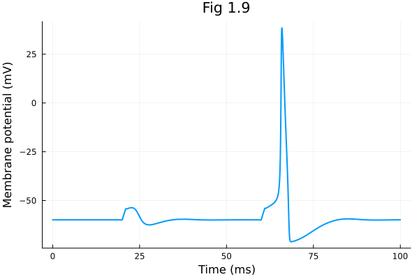
p2 = plot(sol, idxs = [m, h, n], xlabel="")
p3 = plot(sol, idxs = iStim, xlabel="Time (ms)", ylabel="Current (uA/cm^2)", label="Stimulation current", legend=:left)
plot(p1, p2, p3, layout=(3, 1), size=(600, 900), leftmargin=5*Plots.mm)

---

This notebook was generated using Literate.jl.