using ModelingToolkit
using Catalyst
using OrdinaryDiffEq
using SteadyStateDiffEq
using Plots
Plots.default(linewidth=2)Fig 6.3
Two component pathway
rn = @reaction_network begin
    (k1 * L, km1), R <--> RL
    k2, P + RL --> Ps + RL
    k3, Ps--> P
end
\[ \begin{align*} \mathrm{R} &\xrightleftharpoons[\mathtt{km1}]{L \mathtt{k1}} \mathrm{\mathtt{RL}} \\ \mathrm{P} + \mathrm{\mathtt{RL}} &\xrightarrow{\mathtt{k2}} \mathrm{\mathtt{Ps}} + \mathrm{\mathtt{RL}} \\ \mathrm{\mathtt{Ps}} &\xrightarrow{\mathtt{k3}} \mathrm{P} \end{align*} \]
setdefaults!(rn, [
    :R => 3.,
    :RL => 0.,
    :P => 8.0,
    :Ps => 0.,
    :L => 0.,
    :k1 => 5.,
    :km1 => 1.,
    :k2 => 6.,
    :k3 => 2.,
])

@independent_variables t
@unpack L = rn
discrete_events = [[1.0] => [L~3.0], [3.0] => [L~0.0]]

osys = convert(ODESystem, rn; discrete_events, remove_conserved = true) |> structural_simplify
\[ \begin{align} \frac{\mathrm{d} P\left( t \right)}{\mathrm{d}t} &= \mathtt{k3} \left( - P\left( t \right) + \Gamma_{2} \right) - \mathtt{k2} \left( - R\left( t \right) + \Gamma_{1} \right) P\left( t \right) \\ \frac{\mathrm{d} R\left( t \right)}{\mathrm{d}t} &= \mathtt{km1} \left( - R\left( t \right) + \Gamma_{1} \right) - L \mathtt{k1} R\left( t \right) \end{align} \]
equations(osys)\[ \begin{align} \frac{\mathrm{d} P\left( t \right)}{\mathrm{d}t} &= \mathtt{k3} \left( - P\left( t \right) + \Gamma_{2} \right) - \mathtt{k2} \left( - R\left( t \right) + \Gamma_{1} \right) P\left( t \right) \\ \frac{\mathrm{d} R\left( t \right)}{\mathrm{d}t} &= \mathtt{km1} \left( - R\left( t \right) + \Gamma_{1} \right) - L \mathtt{k1} R\left( t \right) \end{align} \]
Fig. 6.3 A
tspan = (0., 10.)
prob = ODEProblem(osys, [], tspan, [])
sol = solve(prob)
retcode: Success
Interpolation: 3rd order Hermite
t: 51-element Vector{Float64}:
0.0
9.999999999999999e-5
0.0010999999999999998
0.011099999999999997
0.11109999999999996
1.0
1.0
1.0463687845335854
1.0687821871454328
1.110257175110315
⋮
5.717160539667416
6.1011479186475315
6.5290797493093065
7.006355545327002
7.540553625680684
8.142549043858686
8.828818546386866
9.625182680128827
10.0
u: 51-element Vector{Vector{Float64}}:
[8.0, 3.0]
[8.0, 3.0]
[8.0, 3.0]
[8.0, 3.0]
[8.0, 3.0]
[8.0, 3.0]
[8.0, 3.0]
[6.408338177835746, 1.5269184341495887]
[5.196367770807915, 1.1232765241899925]
[3.307609564576659, 0.6694325732148665]
⋮
[4.585874519631835, 2.8142005246723847]
[5.222764915894311, 2.87344447186153]
[5.859931006576906, 2.9175039423599265]
[6.454538443292145, 2.948813427740215]
[6.966562707384311, 2.969997376980437]
[7.368960043804987, 2.9835668143490177]
[7.654328099232811, 2.991726411815315]
[7.834374287877935, 2.996268501614989]
[7.883912265610946, 2.9974349114353545]@unpack RL, Ps = osys
fig = plot(sol, idxs=[RL, Ps], labels= ["RL" "P*"])
plot!(fig, t -> 3 * (1<=t<=3), label="Ligand", line=(:black, :dash), linealpha=0.7)
plot!(fig, title="Fig. 6.3 (A)", xlabel="Time", ylabel="Concentration")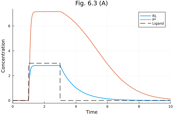
Fig 6.3 B
@unpack RL, Ps = osys
lrange = 0:0.01:1

prob_func = (prob, i, repeat) -> remake(prob, p=[L => lrange[i]])
prob = SteadyStateProblem(osys, [], [])
trajectories = length(lrange)
alg = DynamicSS(Rodas5())
eprob = EnsembleProblem(prob; prob_func)
sim = solve(eprob, alg; trajectories, abstol=1e-10, reltol=1e-10)

pstar = map(s->s[Ps], sim)
rl = map(s->s[RL], sim)
plot(lrange, [pstar rl], label=["P*" "RL"], title="Fig. 6.3 (B)",
xlabel="Ligand", ylabel="Steady-state concentration", xlims=(0, 1), ylims=(0, 8))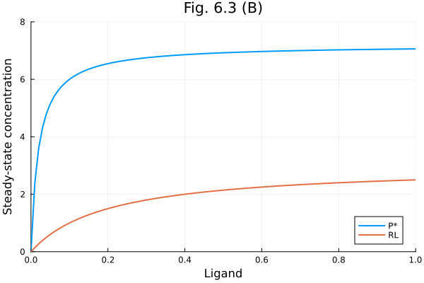
This notebook was generated using Literate.jl.