using OrdinaryDiffEq
using ComponentArrays
using SimpleUnPack
using Plots
Plots.default(linewidth=2)Fig 2.11, 2.12, 2.13, 2.14
Model reduction of ODE metabolic networks.
function model211!(du, u, p, t)
    @unpack k0, k1, km1, k2 = p
    @unpack A, B = u
    v0 = k0
    v1 = k1 * A - km1 * B
    v2 = k2 * B
    du.A = v0 - v1
    du.B = v1 - v2
    nothing
end
model211! (generic function with 1 method)ps211 = ComponentArray(
k0 = 0.0,
k1 = 9.0,
km1 = 12.0,
k2 = 2.0
)
u0 = ComponentArray(
A = 0.0,
B = 10.0
)
tend = 3.0
prob211 = ODEProblem(model211!, u0, tend, ps211)ODEProblem with uType ComponentArrays.ComponentVector{Float64, Vector{Float64}, Tuple{ComponentArrays.Axis{(A = 1, B = 2)}}} and tType Float64. In-place: true Non-trivial mass matrix: false timespan: (0.0, 3.0) u0: ComponentVector{Float64}(A = 0.0, B = 10.0)
@time sol211 = solve(prob211, Tsit5()) 2.210203 seconds (8.23 M allocations: 413.843 MiB, 3.17% gc time, 100.00% compilation time)retcode: Success
Interpolation: specialized 4th order "free" interpolation
t: 35-element Vector{Float64}:
0.0
8.33250002662905e-6
9.165750029291953e-5
0.0009249075029558242
0.0049255520098868185
0.012950994848397006
0.0242033909176605
0.0386770307390286
0.056874831424329884
0.0788503957456076
⋮
1.8976419863766623
2.04653471747305
2.199447644522893
2.3553401128119527
2.512411490644732
2.6691958789164265
2.8250502965479143
2.9800392317414297
3.0
u: 35-element Vector{ComponentArrays.ComponentVector{Float64, Vector{Float64}, Tuple{ComponentArrays.Axis{(A = 1, B = 2)}}}}:
ComponentVector{Float64}(A = 0.0, B = 10.0)
ComponentVector{Float64}(A = 0.0009998041949395534, B = 9.99883355552422)
ComponentVector{Float64}(A = 0.010987314386434823, B = 9.987180710981443)
ComponentVector{Float64}(A = 0.10981641889273347, B = 9.871804396920822)
ComponentVector{Float64}(A = 0.5587746014145984, B = 9.345993049721082)
ComponentVector{Float64}(A = 1.3433471992221453, B = 8.419063000156342)
ComponentVector{Float64}(A = 2.223361128230487, B = 7.361953780480143)
ComponentVector{Float64}(A = 3.060323104867132, B = 6.3276211361048285)
ComponentVector{Float64}(A = 3.771157223127691, B = 5.404354642864228)
ComponentVector{Float64}(A = 4.2896904503815785, B = 4.665729178966642)
⋮
ComponentVector{Float64}(A = 1.2038103571646983, B = 0.8220175368337546)
ComponentVector{Float64}(A = 1.066905753496713, B = 0.7284268312399803)
ComponentVector{Float64}(A = 0.9424542249339941, B = 0.6434317390046563)
ComponentVector{Float64}(A = 0.8304907306491592, B = 0.5670029920694487)
ComponentVector{Float64}(A = 0.7311216458221683, B = 0.49918307682576957)
ComponentVector{Float64}(A = 0.6437926931467843, B = 0.4395767934853836)
ComponentVector{Float64}(A = 0.5673269320456524, B = 0.3873753245348507)
ComponentVector{Float64}(A = 0.5002984513219358, B = 0.34160833595345247)
ComponentVector{Float64}(A = 0.49230199214987075, B = 0.33607801700657547)
Fig 2.11
plot(
    sol211,
    xlabel="Time (AU)",
    ylabel="Concentration (AU)",
    title="Fig. 2.11 (Full model)",
    labels=["A" "B"]
)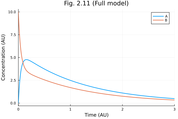
Figure 2.12
Rapid equilibrium assumption
_a212(u, p, t) =  u.C * p.km1 / (p.km1 + p.k1)
function model212!(du, u, p, t)
    @unpack k0, k2 = p
    @unpack C = u
    A = _a212(u, p, t)
    B = C - A
    v0 = k0
    v2 = k2 * B
    du.C = v0 - v2
    nothing
end
model212! (generic function with 1 method)tend = 3.0
prob212 = ODEProblem(model212!, ComponentArray(C = sum(u0)), tend, ps211)ODEProblem with uType ComponentArrays.ComponentVector{Float64, Vector{Float64}, Tuple{ComponentArrays.Axis{(C = 1,)}}} and tType Float64. In-place: true Non-trivial mass matrix: false timespan: (0.0, 3.0) u0: ComponentVector{Float64}(C = 10.0)
@time sol212 = solve(prob212, Tsit5()) 2.071876 seconds (7.96 M allocations: 400.327 MiB, 4.16% gc time, 100.00% compilation time)retcode: Success
Interpolation: specialized 4th order "free" interpolation
t: 9-element Vector{Float64}:
0.0
0.10313309318586757
0.3753972361702897
0.7370512456211995
1.167737125797318
1.6758020636903974
2.2474174188288836
2.8795734914073643
3.0
u: 9-element Vector{ComponentArrays.ComponentVector{Float64, Vector{Float64}, Tuple{ComponentArrays.Axis{(C = 1,)}}}}:
ComponentVector{Float64}(C = 10.0)
ComponentVector{Float64}(C = 9.153948340781719)
ComponentVector{Float64}(C = 7.248655848460791)
ComponentVector{Float64}(C = 5.3165629074890655)
ComponentVector{Float64}(C = 3.6754225790588713)
ComponentVector{Float64}(C = 2.3778226155035846)
ComponentVector{Float64}(C = 1.4567854018333564)
ComponentVector{Float64}(C = 0.8473770113337553)
ComponentVector{Float64}(C = 0.7642714199479215)
fig = plot(sol211, line=(:dash, 1), label=["A (full solution)" "B (full solution)"])
ts = sol212.t
cs = sol212[1, :]
as = _a212.(sol212.u, Ref(ps211), ts)
bs = cs .- as
plot!(fig, ts, [as bs], label=["A (rapid equilibrium)" "B (rapid equilibrium)"])

plot!(fig,
    title="Fig. 2.12 (Rapid equilibrium model)",
    xlabel="Time (AU)",
    ylabel="Concentration (AU)"
)

fig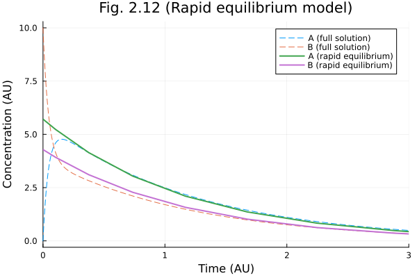
Figure 2.13
Rapid equilibrium (take 2)
When another set of parameters is not suitable for rapid equilibrium assumption.
ps213 = ComponentArray(k0 = 9.0, k1 = 20.0, km1 = 12.0, k2 = 2.0)
u0 = ComponentArray(A = 8.0, B = 4.0)
tend = 3.0

@time sol213full = solve(ODEProblem(model211!, u0, tend, ps213), Tsit5())
@time sol213re = solve(ODEProblem(model212!, ComponentArray(C = sum(u0)), tend, ps213), Tsit5())
0.000150 seconds (779 allocations: 32.641 KiB)
0.000196 seconds (315 allocations: 13.000 KiB)retcode: Success
Interpolation: specialized 4th order "free" interpolation
t: 9-element Vector{Float64}:
0.0
0.10985788520382275
0.3514885215968111
0.6586777912438853
1.0393785582716237
1.4959514209075846
2.0369831593840857
2.672183436982096
3.0
u: 9-element Vector{ComponentArrays.ComponentVector{Float64, Vector{Float64}, Tuple{ComponentArrays.Axis{(C = 1,)}}}}:
ComponentVector{Float64}(C = 12.0)
ComponentVector{Float64}(C = 11.384108095813618)
ComponentVector{Float64}(C = 10.293352240189929)
ComponentVector{Float64}(C = 9.307008837373226)
ComponentVector{Float64}(C = 8.509173268418104)
ComponentVector{Float64}(C = 7.939847552423305)
ComponentVector{Float64}(C = 7.576224445585626)
ComponentVector{Float64}(C = 7.370083403215763)
ComponentVector{Float64}(C = 7.312901875215382)
fig = plot(sol213full, line=(:dash, 1), label=["A (full solution)" "B (full solution)"])
ts = sol213re.t
cs = sol213re[1, :]
as = _a212.(sol213re.u, Ref(ps213), ts)
bs = cs .- as
plot!(fig, ts, [as bs], label=["A (rapid equilibrium)" "B (rapid equilibrium)"])
plot!(fig,
    title="Fig. 2.13 (Rapid equilibrium model)",
    xlabel="Time (AU)",
    ylabel="Concentration (AU)"
)

fig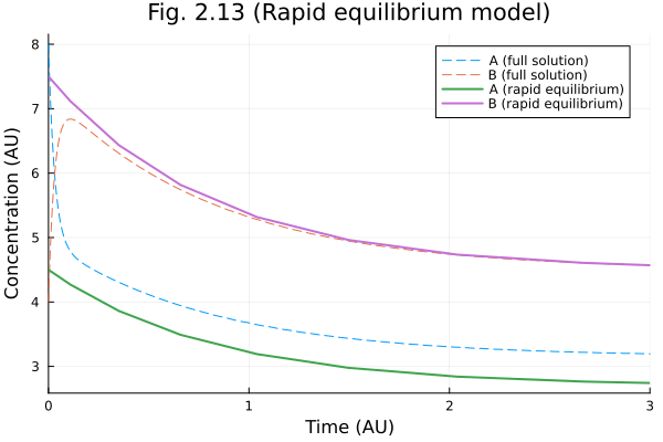
Figure 2.14 : QSSA
Quasi-steady state assumption on species A
_a214(u, p, t) = (p.k0 + p.km1 * u.B) / p.k1
_u0214(u0, p) = (p.k1 * u0 - p.k0) / (p.k1 + p.km1)
function model214!(du, u, p, t)
    @unpack k0, k1, km1, k2 = p
    @unpack B = u
    A = _a214(u, p, t)
    du.B = k1 * A - (km1 + k2) * B
    nothing
end

ps214 = ps213
u0214= ComponentArray(B = _u0214(sum(u0), ps214))
ComponentVector{Float64}(B = 7.21875)
Solve QSSA model
@time sol214 = solve(ODEProblem(model214!, u0214, tend, ps214), Tsit5())

fig = plot(sol213full, line=(:dash), label=["A (full solution)" "B (full solution)"])
ts = sol214.t
as = _a214.(sol214.u, Ref(ps214), ts)
bs = sol214[1, :]
plot!(fig, ts, [as bs], label=["A (QSSA)" "B (QSSA)"])
plot!(fig,
    xlabel="Time (AU)",
    ylabel="Concentration (AU)",
    title="Figure 2.14: Ref vs QSSA",
    xlims=(0.0, tend)
)
2.068636 seconds (8.05 M allocations: 406.281 MiB, 2.23% gc time, 99.97% compilation time)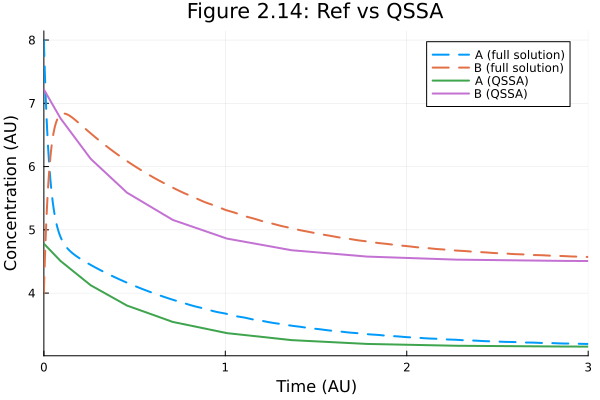
This notebook was generated using Literate.jl.