Solving differential equations in Julia

Standard procedures

• Define a model function representing the right-hand-side (RHS) of the system.

  • Out-of-place form: f(u, p, t) where u is the state variable(s), p is the parameter(s), and t is the independent variable (usually time). The output is the right hand side (RHS) of the differential equation system.

  • In-place form: f!(du, u, p, t), where the output is saved to du. The rest is the same as the out of place form. The in-place form has potential performance benefits since it allocates less than the out-of-place (f(u, p, t)) counterpart.

  • Using ModelingToolkit.jl : define equations and build an ODE system.

• Initial conditions (u0) for the state variable(s).

• (Optional) define parameter(s) p.

• Define a problem (e.g. ODEProblem) using the modeling function (f), initial conditions (u0), simulation time span (tspan == (tstart, tend)), and parameter(s) p.

• Solve the problem by calling solve(prob).

Solve ODEs using OrdinaryDiffEq.jl

Documentation: https://docs.sciml.ai/DiffEqDocs/stable/

Single variable: Exponential decay model

The concentration of a decaying nuclear isotope could be described as an exponential decay:

\[ \frac{d}{dt}C(t) = - \lambda C(t) \]

State variable

• \(C(t)\): The concentration of a decaying nuclear isotope.

Parameter

• \(\lambda\): The rate constant of decay. The half-life \(t_{\frac{1}{2}} = \frac{ln2}{\lambda}\)

using OrdinaryDiffEq
using Plots
Plots.default(linewidth=2)

The model function is the 3-argument out-of-place form, f(u, p, t).

decay(u, p, t) = p * u

p = -1.0            ## Rate of exponential decay
u0 = 1.0            ## Initial condition
tspan = (0.0, 2.0)  ## Start time and end time

prob = ODEProblem(decay, u0, tspan, p)
sol = solve(prob)

retcode: Success
Interpolation: 3rd order Hermite
t: 8-element Vector{Float64}:
 0.0
 0.10001999200479662
 0.34208427066999536
 0.6553980136343391
 1.0312652525315806
 1.4709405856363595
 1.9659576669700232
 2.0
u: 8-element Vector{Float64}:
 1.0
 0.9048193287657775
 0.7102883621328674
 0.5192354400036404
 0.3565557657699655
 0.22970979078638265
 0.1400224727245278
 0.13533600284008826

Solution at time t=1.0 (with interpolation)

sol(1.0)

0.3678796381978344

Time points

sol.t

8-element Vector{Float64}:
 0.0
 0.10001999200479662
 0.34208427066999536
 0.6553980136343391
 1.0312652525315806
 1.4709405856363595
 1.9659576669700232
 2.0

Solutions at corresponding time points

sol.u

8-element Vector{Float64}:
 1.0
 0.9048193287657775
 0.7102883621328674
 0.5192354400036404
 0.3565557657699655
 0.22970979078638265
 0.1400224727245278
 0.13533600284008826

Visualize the solution

plot(sol)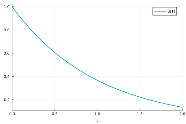

Three variables: The SIR model

The SIR model describes the spreading of an contagious disease can be described by the SIR model:

\[\begin{split} \begin{align} \frac{d}{dt}S(t) &= - \beta S(t)I(t) \\ \frac{d}{dt}I(t) &= \beta S(t)I(t) - \gamma I(t) \\ \frac{d}{dt}R(t) &= \gamma I(t) \end{align} \end{split}\]

State variables

• \(S(t)\) : the fraction of susceptible people

• \(I(t)\) : the fraction of infectious people

• \(R(t)\) : the fraction of recovered (or removed) people

Parameters

• \(\beta\) : the rate of infection when susceptible and infectious people meet

• \(\gamma\) : the rate of recovery of infectious people

using OrdinaryDiffEq
using Plots
Plots.default(linewidth=2)

SIR model (in-place form can save array allocations and thus faster)

function sir!(du, u, p, t)
    s, i, r = u
    β, γ = p
    v1 = β * s * i
    v2 = γ * i
    du[1] = -v1
    du[2] = v1 - v2
    du[3] = v2
    return nothing
end

sir! (generic function with 1 method)

p = (β=1.0, γ=0.3)
u0 = [0.99, 0.01, 0.00]
tspan = (0.0, 20.0)
prob = ODEProblem(sir!, u0, tspan, p)
sol = solve(prob)

retcode: Success
Interpolation: 3rd order Hermite
t: 17-element Vector{Float64}:
  0.0
  0.08921318693905476
  0.3702862715172094
  0.7984257132319627
  1.3237271485666187
  1.991841832691831
  2.7923706947355837
  3.754781614278828
  4.901904318934307
  6.260476636498209
  7.7648912410433075
  9.39040980993922
 11.483861023017885
 13.372369854616487
 15.961357172044833
 18.681426667664056
 20.0
u: 17-element Vector{Vector{Float64}}:
 [0.99, 0.01, 0.0]
 [0.9890894703413342, 0.010634484617786016, 0.00027604504087978485]
 [0.9858331594901347, 0.012901496825852227, 0.0012653436840130792]
 [0.9795270529591532, 0.017282420996456258, 0.003190526044390598]
 [0.9689082167415561, 0.024631267034445452, 0.006460516223998509]
 [0.9490552312363142, 0.03827338797605376, 0.012671380787632129]
 [0.911862947533394, 0.06347250098224955, 0.024664551484356523]
 [0.8398871089274514, 0.11078176031568526, 0.04933113075686341]
 [0.707584206802473, 0.19166147882272797, 0.10075431437479916]
 [0.5081460287219878, 0.2917741934147055, 0.2000797778633069]
 [0.31213222024414106, 0.3415879120018043, 0.34627986775405484]
 [0.1821568309636563, 0.309998313415639, 0.5078448556207048]
 [0.10427205468919257, 0.2206111401113331, 0.6751168051994745]
 [0.07386737407725885, 0.14760143051851196, 0.7785311954042293]
 [0.05545028910907742, 0.07997076922865369, 0.864578941662269]
 [0.04733499069589219, 0.040605653213833574, 0.9120593560902743]
 [0.04522885458929347, 0.02905741611081477, 0.9257137292998918]

Visualize the solution

plot(sol, label=["S" "I" "R"], legend=:right)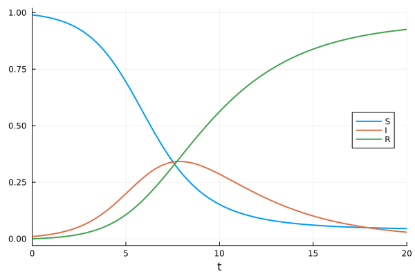

Using ModelingToolkit.jl (recommended)

ModelingToolkit.jl is a high-level package for symbolic-numeric modeling and simulation in the Julia ecosystem.

using ModelingToolkit
using OrdinaryDiffEq
using Plots
Plots.default(linewidth=2)

Exponential decay model

@independent_variables t    ## Time
@parameters λ               ## Decaying rate constant
@variables C(t)             ## Time and concentration
D = Differential(t)         ## Differential operator

Differential(t)

Define an ODE with equations

eqs = [D(C) ~ -λ * C]
@mtkbuild decaySys = ODESystem(eqs, t)

\[ \begin{align} \frac{\mathrm{d} C\left( t \right)}{\mathrm{d}t} &= - C\left( t \right) \lambda \end{align} \]

u0 = [C => 1.0]
p = [λ => 1.0]
tspan = (0.0, 2.0)

prob = ODEProblem(decaySys, u0, tspan, p)
sol = solve(prob)
plot(sol)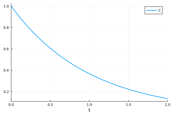

SIR model

using OrdinaryDiffEq
using ModelingToolkit
using Plots
Plots.default(linewidth=2)

@independent_variables t
@parameters β γ
@variables s(t) i(t) r(t)
D = Differential(t)

eqs = [
    D(s) ~ -β * s * i,
    D(i) ~ β * s * i - γ * i,
    D(r) ~ γ * i
]

@mtkbuild sirSys = ODESystem(eqs, t)

\[\begin{split} \begin{align} \frac{\mathrm{d} i\left( t \right)}{\mathrm{d}t} &= - i\left( t \right) \gamma + i\left( t \right) s\left( t \right) \beta \\ \frac{\mathrm{d} r\left( t \right)}{\mathrm{d}t} &= i\left( t \right) \gamma \\ \frac{\mathrm{d} s\left( t \right)}{\mathrm{d}t} &= - i\left( t \right) s\left( t \right) \beta \end{align} \end{split}\]

p = [β => 1.0, γ => 0.3]
u0 = [s => 0.99, i => 0.01, r => 0.00]
tspan = (0.0, 20.0)

prob = ODEProblem(sirSys, u0, tspan, p)
sol = solve(prob)

plot(sol)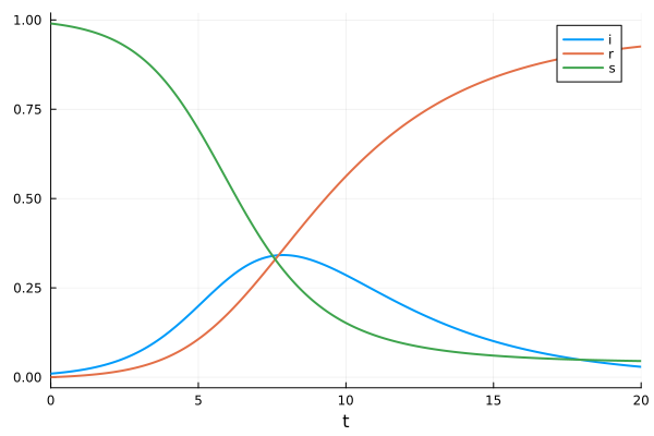

Lorenz system

The Lorenz system is a system of ordinary differential equations having chaotic solutions for certain parameter values and initial conditions. (Wikipedia)

\[\begin{split} \begin{align} \frac{dx}{dt} &= \sigma(y-x) \\ \frac{dy}{dt} &= x(\rho - z) -y \\ \frac{dz}{dt} &= xy - \beta z \end{align} \end{split}\]

using OrdinaryDiffEq
using ModelingToolkit
using Plots
Plots.default(linewidth=2)

Building the model is wrapped in a function

function build_lorentz(; name)
    @parameters begin
        σ = 10.0
        ρ = 28.0
        β = 8 / 3
    end

    @independent_variables t
    @variables begin
        x(t) = 1.0    ## Independent variable (time)
        y(t) = 0.0    ## Independent variable (time)
        z(t) = 0.0    ## Independent variable (time)
    end

    D = Differential(t)

    eqs = [
        D(x) ~ σ * (y - x),
        D(y) ~ x * (ρ - z) - y,
        D(z) ~ x * y - β * z
    ]

    sys = ODESystem(eqs, t; name)
    return sys
end

build_lorentz (generic function with 1 method)

tspan = (0.0, 100.0)
@mtkbuild sys = build_lorentz()
prob = ODEProblem(sys, [], tspan, [])
sol = solve(prob)

retcode: Success
Interpolation: 3rd order Hermite
t: 1325-element Vector{Float64}:
   0.0
   3.5678604836301404e-5
   0.0003924646531993154
   0.003262407732952926
   0.009058075632950364
   0.01695646917889552
   0.027689958632766257
   0.04185634991045167
   0.06024041181372633
   0.08368541086439041
   ⋮
  99.49018875318062
  99.54862803586417
  99.6145902246956
  99.6844772275333
  99.76689729728005
  99.85118113701569
  99.9277902563632
  99.99633045999587
 100.0
u: 1325-element Vector{Vector{Float64}}:
 [1.0, 0.0, 0.0]
 [0.9996434557625105, 0.0009988049817849058, 1.781434788799208e-8]
 [0.9961045497425811, 0.010965399721242457, 2.146955365838907e-6]
 [0.9693591636090403, 0.08977060609621872, 0.0001438018323641714]
 [0.9242043615200224, 0.24228912476918024, 0.001046162329727883]
 [0.8800455859164964, 0.4387364554855289, 0.003424259429099474]
 [0.8483309846305274, 0.6915629338584358, 0.008487624633044172]
 [0.8495036661237968, 1.0145426239346456, 0.018212089206688865]
 [0.9139069582771231, 1.4425599843977082, 0.036693822160421524]
 [1.0888638105810242, 2.0523265477022825, 0.07402573342120332]
 ⋮
 [-0.9940591016433658, -2.8817300441171474, 21.71504831029168]
 [-1.928880273667646, -3.388601591720348, 18.833364484674814]
 [-2.9751110649395445, -4.815097635912501, 16.400650729866644]
 [-4.625266725547489, -7.632665256875718, 15.107297022943598]
 [-7.9439838455455565, -13.030768900739405, 16.94732621617739]
 [-12.5991630525995, -17.606167341053442, 26.084946638181943]
 [-14.18564328360291, -12.357314081660197, 36.407114774499064]
 [-10.767406782468159, -3.6671228558902, 36.59399970621433]
 [-10.505291991542054, -3.323107353088182, 36.373367127901254]

x-y-z time-series

plot(sol)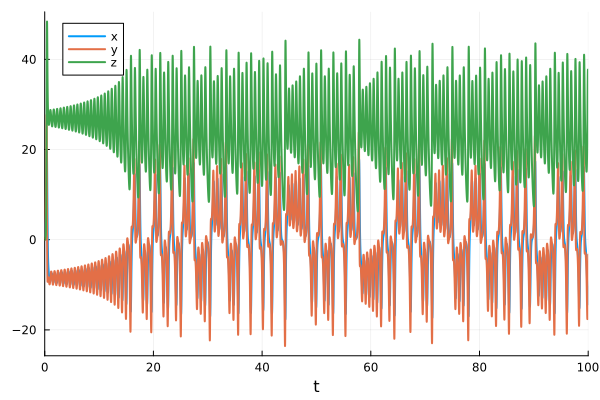

y-t plot

plot(sol, idxs=[sys.y])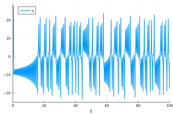

idxs=(sys.x, sys.y, sys.z) makes a phase plot.

plot(sol, idxs=(sys.x, sys.y, sys.z), label=false, size=(600, 600))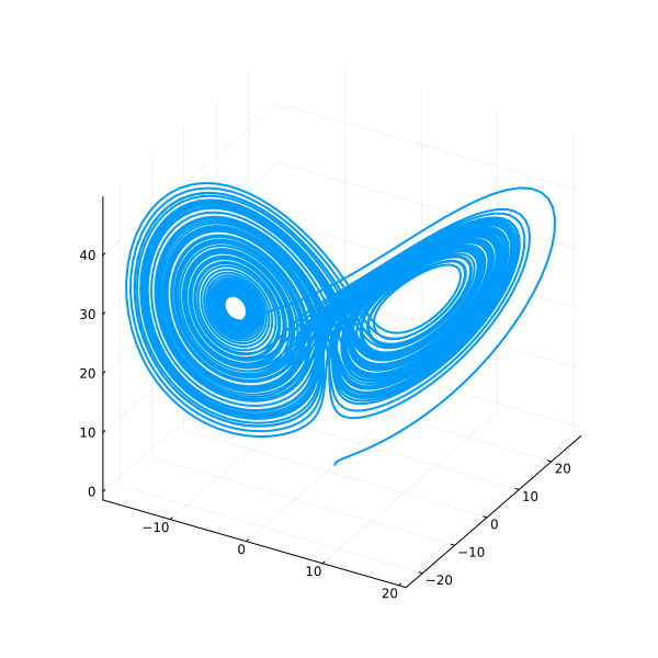

Saving simulation results

using DataFrames
using CSV

df = DataFrame(sol)
CSV.write("lorenz.csv", df)
rm("lorenz.csv")

Catalyst.jl

Catalyst.jl is a domain-specific language (DSL) package to simulate chemical reaction networks.

using OrdinaryDiffEq
using Catalyst
using Plots
Plots.default(linewidth=2)

Exponential decay model

decay_rn = @reaction_network begin
    λ, C --> 0
end

\[ \begin{align*} \mathrm{C} &\xrightarrow{\lambda} \varnothing \end{align*} \]

p = [:λ => 1.0]
u0 = [:C => 1.0]
tspan = (0.0, 2.0)

prob = ODEProblem(decay_rn, u0, tspan, p)
sol = solve(prob)

retcode: Success
Interpolation: 3rd order Hermite
t: 8-element Vector{Float64}:
 0.0
 0.10001999200479662
 0.34208427066999536
 0.6553980136343391
 1.0312652525315806
 1.4709405856363595
 1.9659576669700232
 2.0
u: 8-element Vector{Vector{Float64}}:
 [1.0]
 [0.9048193287657775]
 [0.7102883621328674]
 [0.5192354400036404]
 [0.3565557657699655]
 [0.22970979078638265]
 [0.1400224727245278]
 [0.13533600284008826]

plot(sol, title="Exponential Decay")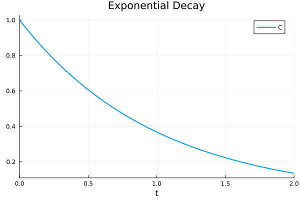

SIR model

sir_rn = @reaction_network begin
    β, S + I --> 2I
    γ, I --> R
end

\[\begin{split} \begin{align*} \mathrm{S} + \mathrm{I} &\xrightarrow{\beta} 2 \mathrm{I} \\ \mathrm{I} &\xrightarrow{\gamma} \mathrm{R} \end{align*} \end{split}\]

Extract the symbols for later use

@unpack β, γ, S, I, R = sir_rn

p = [β => 1.0, γ => 0.3]
u0 = [S => 0.99, I => 0.01, R => 0.00]
tspan = (0.0, 20.0)

prob = ODEProblem(sir_rn, u0, tspan, p)
sol = solve(prob)

retcode: Success
Interpolation: 3rd order Hermite
t: 17-element Vector{Float64}:
  0.0
  0.08921318693905476
  0.3702862715172094
  0.7984257132319627
  1.3237271485666187
  1.991841832691831
  2.7923706947355837
  3.754781614278828
  4.901904318934307
  6.260476636498209
  7.7648912410433075
  9.39040980993922
 11.483861023017885
 13.372369854616487
 15.961357172044833
 18.681426667664056
 20.0
u: 17-element Vector{Vector{Float64}}:
 [0.99, 0.01, 0.0]
 [0.9890894703413342, 0.010634484617786016, 0.00027604504087978485]
 [0.9858331594901347, 0.012901496825852227, 0.0012653436840130792]
 [0.9795270529591532, 0.017282420996456258, 0.003190526044390598]
 [0.9689082167415561, 0.024631267034445452, 0.006460516223998509]
 [0.9490552312363142, 0.03827338797605376, 0.012671380787632129]
 [0.911862947533394, 0.06347250098224955, 0.024664551484356523]
 [0.8398871089274514, 0.11078176031568526, 0.04933113075686341]
 [0.707584206802473, 0.19166147882272797, 0.10075431437479916]
 [0.5081460287219878, 0.2917741934147055, 0.2000797778633069]
 [0.31213222024414106, 0.3415879120018043, 0.34627986775405484]
 [0.1821568309636563, 0.309998313415639, 0.5078448556207048]
 [0.10427205468919257, 0.2206111401113331, 0.6751168051994745]
 [0.07386737407725885, 0.14760143051851196, 0.7785311954042293]
 [0.05545028910907742, 0.07997076922865369, 0.864578941662269]
 [0.04733499069589219, 0.040605653213833574, 0.9120593560902743]
 [0.04522885458929347, 0.02905741611081477, 0.9257137292998918]

plot(sol, legend=:right, title="SIR Model")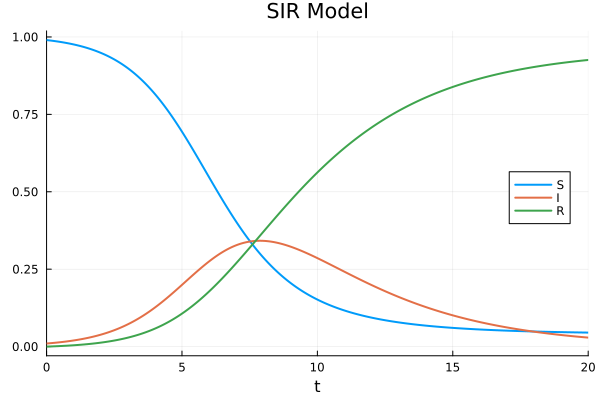

---

This notebook was generated using Literate.jl.