using ComponentArrays
using SimpleUnPack
using OrdinaryDiffEq
using DiffEqCallbacks
using Plots
Plots.default(linewidth=2)Fig 6.14
Model of E. coli chemotaxis signalling pathway
hil(x, k) = x / (k + x)
hil(x, k, n) = hil(x^n, k^n)
function model614!(D, u, p, t)
    @unpack k1, k2, k3, km1, km2, km3, k4, km4, k5, km5, KM1, KM2, L, R, Atotal, Btotal = p
    @unpack Am, AmL, AL, BP = u
    A = Atotal - Am - AmL - AL
    B = Btotal - BP
    v1 = k1 * BP * hil(Am, KM1)
    v2 = k2 * BP * hil(AmL, KM2)
    v3 = km1 * R
    v4 = km2 * R
    v5 = k3 * L * Am - km3 * AmL
    v6 = k4 * L * A - km4 * AL
    v7 = k5 * Am * B - km5 * BP
    D.Am = v3 - v1 - v5
    D.AmL = v4 - v2 + v5
    D.AL = v2 + v6
    D.BP = v7
    nothing
end
model614! (generic function with 1 method)ps614 = ComponentArray(
k1 = 200.0,
k2 = 1.0,
k3 = 1.0,
km1 = 1.0,
km2 = 1.0,
km3 = 1.0,
k4 = 1.0,
km4 = 1.0,
k5 = 0.05,
km5 = 0.005,
KM1 = 1.0,
KM2 = 1.0,
L = 20.0,
R = 1.0,
Atotal = 2.0,
Btotal = 1.0
)
u0614 = ComponentArray(
Am = 0.0360,
AmL = 1.5593,
AL = 0.3504,
BP = 0.2644
)ComponentVector{Float64}(Am = 0.036, AmL = 1.5593, AL = 0.3504, BP = 0.2644)
Events to increase L
affect_L1!(integrator) = integrator.p.L = 40.0
affect_L2!(integrator) = integrator.p.L = 80.0
event_L1 = PresetTimeCallback([10.0], affect_L1!)
event_L2 = PresetTimeCallback([30.0], affect_L2!)
cbs = CallbackSet(event_L1, event_L2)
SciMLBase.CallbackSet{Tuple{}, Tuple{SciMLBase.DiscreteCallback{DiffEqCallbacks.PresetTimeFunction{Vector{Float64}, typeof(SciMLBase.INITIALIZE_DEFAULT), typeof(Main.var"##328".affect_L1!)}, typeof(Main.var"##328".affect_L1!), DiffEqCallbacks.PresetTimeFunction{Vector{Float64}, typeof(SciMLBase.INITIALIZE_DEFAULT), typeof(Main.var"##328".affect_L1!)}, typeof(SciMLBase.FINALIZE_DEFAULT), Nothing, Tuple{}}, SciMLBase.DiscreteCallback{DiffEqCallbacks.PresetTimeFunction{Vector{Float64}, typeof(SciMLBase.INITIALIZE_DEFAULT), typeof(Main.var"##328".affect_L2!)}, typeof(Main.var"##328".affect_L2!), DiffEqCallbacks.PresetTimeFunction{Vector{Float64}, typeof(SciMLBase.INITIALIZE_DEFAULT), typeof(Main.var"##328".affect_L2!)}, typeof(SciMLBase.FINALIZE_DEFAULT), Nothing, Tuple{}}}}((), (SciMLBase.DiscreteCallback{DiffEqCallbacks.PresetTimeFunction{Vector{Float64}, typeof(SciMLBase.INITIALIZE_DEFAULT), typeof(Main.var"##328".affect_L1!)}, typeof(Main.var"##328".affect_L1!), DiffEqCallbacks.PresetTimeFunction{Vector{Float64}, typeof(SciMLBase.INITIALIZE_DEFAULT), typeof(Main.var"##328".affect_L1!)}, typeof(SciMLBase.FINALIZE_DEFAULT), Nothing, Tuple{}}(DiffEqCallbacks.PresetTimeFunction{Vector{Float64}, typeof(SciMLBase.INITIALIZE_DEFAULT), typeof(Main.var"##328".affect_L1!)}([10.0], true, SciMLBase.INITIALIZE_DEFAULT, Main.var"##328".affect_L1!), Main.var"##328".affect_L1!, DiffEqCallbacks.PresetTimeFunction{Vector{Float64}, typeof(SciMLBase.INITIALIZE_DEFAULT), typeof(Main.var"##328".affect_L1!)}([10.0], true, SciMLBase.INITIALIZE_DEFAULT, Main.var"##328".affect_L1!), SciMLBase.FINALIZE_DEFAULT, Bool[1, 1], nothing, ()), SciMLBase.DiscreteCallback{DiffEqCallbacks.PresetTimeFunction{Vector{Float64}, typeof(SciMLBase.INITIALIZE_DEFAULT), typeof(Main.var"##328".affect_L2!)}, typeof(Main.var"##328".affect_L2!), DiffEqCallbacks.PresetTimeFunction{Vector{Float64}, typeof(SciMLBase.INITIALIZE_DEFAULT), typeof(Main.var"##328".affect_L2!)}, typeof(SciMLBase.FINALIZE_DEFAULT), Nothing, Tuple{}}(DiffEqCallbacks.PresetTimeFunction{Vector{Float64}, typeof(SciMLBase.INITIALIZE_DEFAULT), typeof(Main.var"##328".affect_L2!)}([30.0], true, SciMLBase.INITIALIZE_DEFAULT, Main.var"##328".affect_L2!), Main.var"##328".affect_L2!, DiffEqCallbacks.PresetTimeFunction{Vector{Float64}, typeof(SciMLBase.INITIALIZE_DEFAULT), typeof(Main.var"##328".affect_L2!)}([30.0], true, SciMLBase.INITIALIZE_DEFAULT, Main.var"##328".affect_L2!), SciMLBase.FINALIZE_DEFAULT, Bool[1, 1], nothing, ())))tend = 50.0
prob614 = ODEProblem(model614!, u0614, tend, ps614)ODEProblem with uType ComponentArrays.ComponentVector{Float64, Vector{Float64}, Tuple{ComponentArrays.Axis{(Am = 1, AmL = 2, AL = 3, BP = 4)}}} and tType Float64. In-place: true Non-trivial mass matrix: false timespan: (0.0, 50.0) u0: ComponentVector{Float64}(Am = 0.036, AmL = 1.5593, AL = 0.3504, BP = 0.2644)
@time sol614 = solve(prob614, Tsit5(), callback=cbs) 2.594238 seconds (8.62 M allocations: 433.533 MiB, 1.50% gc time, 99.96% compilation time)retcode: Success
Interpolation: specialized 4th order "free" interpolation
t: 1461-element Vector{Float64}:
0.0
0.05177261337107878
0.07855385959151512
0.12183666398224637
0.16755912839346007
0.22428468941141977
0.2855225141764318
0.3443808456113713
0.3983842394766113
0.44861315531808205
⋮
49.80541595578783
49.83246739791603
49.8595188497345
49.886570313305015
49.91362179068935
49.94067327982574
49.967724778652425
49.99477628696323
50.0
u: 1461-element Vector{ComponentArrays.ComponentVector{Float64, Vector{Float64}, Tuple{ComponentArrays.Axis{(Am = 1, AmL = 2, AL = 3, BP = 4)}}}}:
ComponentVector{Float64}(Am = 0.036, AmL = 1.5593, AL = 0.3504, BP = 0.2644)
ComponentVector{Float64}(Am = 0.03599551644359868, AmL = 1.5593077321638846, AL = 0.37866688255554337, BP = 0.2644001586129533)
ComponentVector{Float64}(Am = 0.036020470807065746, AmL = 1.5593036601019372, AL = 0.3848679710225929, BP = 0.2644002262627703)
ComponentVector{Float64}(Am = 0.03602357483180375, AmL = 1.5593077996917124, AL = 0.38976424443741975, BP = 0.2644003553293034)
ComponentVector{Float64}(Am = 0.036024557266477825, AmL = 1.5593126524213565, AL = 0.3918010073395575, BP = 0.26440049294393936)
ComponentVector{Float64}(Am = 0.03602335906401148, AmL = 1.5593191161695759, AL = 0.39267587496843437, BP = 0.2644006650308085)
ComponentVector{Float64}(Am = 0.03601742087981962, AmL = 1.5593271372524034, AL = 0.39294668632521823, BP = 0.26440085335001684)
ComponentVector{Float64}(Am = 0.03600312361706433, AmL = 1.5593370647775553, AL = 0.39301266521513545, BP = 0.2644010389765156)
ComponentVector{Float64}(Am = 0.035990749909848324, AmL = 1.559345723242336, AL = 0.3930251683035488, BP = 0.26440120897182123)
ComponentVector{Float64}(Am = 0.03599177356524357, AmL = 1.5593499206371084, AL = 0.3930275248033512, BP = 0.2644013605060869)
⋮
ComponentVector{Float64}(Am = 0.03538463374319951, AmL = 3.6230816930479857, AL = -1.635427372060331, BP = 0.2625847165638323)
ComponentVector{Float64}(Am = 0.03538472243868478, AmL = 3.6230914504559424, AL = -1.6354371294682857, BP = 0.2625844739849415)
ComponentVector{Float64}(Am = 0.035384810577769106, AmL = 3.6231011380283826, AL = -1.635446817040726, BP = 0.26258423153851357)
ComponentVector{Float64}(Am = 0.035384898175325516, AmL = 3.6231107564759117, AL = -1.6354564354882557, BP = 0.2625839892239576)
ComponentVector{Float64}(Am = 0.035384985246179966, AmL = 3.623120306501673, AL = -1.6354659855140192, BP = 0.2625837470406884)
ComponentVector{Float64}(Am = 0.035385071786679746, AmL = 3.623129788811437, AL = -1.6354754678237824, BP = 0.2625835049881684)
ComponentVector{Float64}(Am = 0.03538515779310343, AmL = 3.6231392041037123, AL = -1.6354848831160578, BP = 0.2625832630658657)
ComponentVector{Float64}(Am = 0.035385243269955485, AmL = 3.6231485530653074, AL = -1.635494232077652, BP = 0.26258302127323485)
ComponentVector{Float64}(Am = 0.035375858274519535, AmL = 3.6231561984048746, AL = -1.6355018774172194, BP = 0.2625829772715587)
plot(sol614, idxs=[1], title="Fig 6.14", xlabel="Time", ylabel="Active CheA ([Am])", ylims=(0.01, 0.04), legend=false)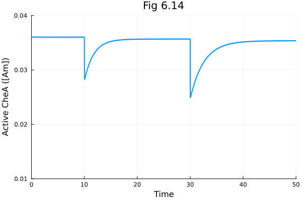
This notebook was generated using Literate.jl.
Back to top