CaMK parameter fitting - NRVM CaMKII model

Fitting CaMKII parameters to experimental decay rates.

using ModelingToolkit
using ModelingToolkit: t_nounits as t, D_nounits as D
using OrdinaryDiffEq
using Optimization
using OptimizationOptimJL
using OptimizationLBFGSB
using ADTypes
using ForwardDiff
using DiffEqCallbacks
using CurveFit
using Plots
using LinearAlgebra
using Model
using Model: second

Experimental data¶

CaMKII activity decay times after 1Hz pacing for 15.0, 30.0, 60.0, 90.0 seconds.

pacing_durations = [15.0, 30.0, 60.0, 90.0]
experimental_taus = [16.48, 16.73, 17.65, 18.08]

4-element Vector{Float64}:
 16.48
 16.73
 17.65
 18.08

Simplified calcium transient¶

We use a fitted model for calcium transients to speed up CaMKII parameter fitting.

stimstart = 0.0second
stimend = 100.0second
tend = stimend + 50.0second
alg = TRBDF2()
@time "Building ODE system" sys = Model.DEFAULT_SYS
@time "Building ODE problem" prob = ODEProblem(sys, [], tend)
@unpack Istim = sys
cb = Model.build_stim_callbacks(Istim, stimend; period=1second, starttime=stimstart)
@time "Solving ODE problem" sol = solve(prob, alg, callback=cb);

Building ODE system: 0.000010 seconds
Building ODE problem: 32.998195 seconds (35.84 M allocations: 2.480 GiB, 2.68% gc time, 99.19% compilation time: 37% of which was recompilation)
Solving ODE problem: 3.800402 seconds (4.99 M allocations: 716.989 MiB, 3.16% gc time, 69.01% compilation time)

Fit the calcium transient curve¶

Using Rational polynomial fit to fit the calcium transient curve.

ts = range(0.0, 2.0second, step=0.01second)
cai = sol(ts .+ 100.0second, idxs=sys.Cai_mean).u

prob = CurveFitProblem(ts, cai)
n_num = 7
n_den = 7
@time fit = solve(prob, RationalPolynomialFitAlgorithm(n_num, n_den))
println("Numerator coefficients: ", fit.u[1:n_num+1])
println("Denominator coefficients: ", vcat(1.0, fit.u[n_num+2:end]))
println("RMSE: ", mse(fit) |> sqrt)

  6.038685 seconds (6.83 M allocations: 487.330 MiB, 1.59% gc time, 97.72% compilation time)
Numerator coefficients: [0.23701283514127058, -0.000934339764671451, -5.369342124978498e-6, 2.8926386498830786e-8, 2.5707796158290392e-11, -3.7022796256746537e-14, 2.6692630577785824e-17, -1.0324936237251978e-20]
Denominator coefficients: [1.0, -0.011835118981551616, 6.238005037115056e-5, -1.9950567951087674e-7, 4.538682920518767e-10, -3.1735753388971964e-13, 2.0976906224380044e-16, -8.07971681875386e-20]
RMSE: 0.00014843758145121662

Visualization¶

plot(ts, cai, label="Data", line=:solid)
plot!(ts, fit.(ts), label="Fit", line=:dash)
plot!(xlabel="Time (ms)", ylabel="Ca (μM)", title="Calcium transient fitting", size=(800, 400))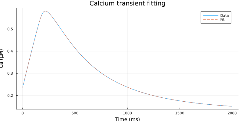

Some discrepancy at rest

ts = range(0.0, 50.0second, step=0.1second)
cai = sol(ts .+ 100.0second, idxs=sys.Cai_mean).u
plot(ts, cai, label="Data", line=:solid)
plot!(ts, fit.(ts), label="Fit", line=:dash)
plot!(xlabel="Time (ms)", ylabel="Ca (μM)", title="Calcium transient fitting", size=(800, 400))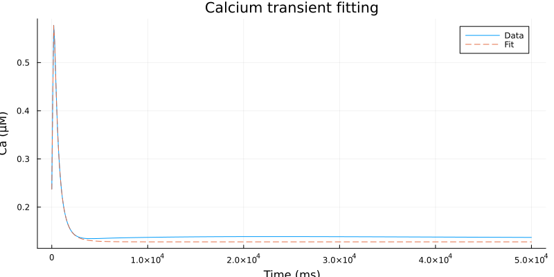

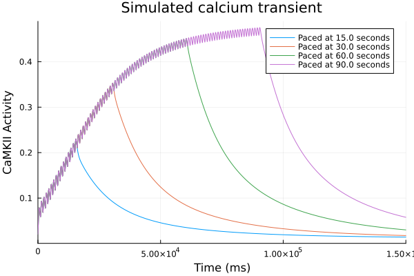
Calcium transient curve¶

Simulated calcium transients fitted against those in the whole model with 1 Hz pacing. (for 0 <= t <= 1000ms). Here we use an implicit time variable tau to track time, and fit the calcium transient curve as a rational polynomial function of tau.

@variables tau(t) Ca(t)

eqs = [
    D(tau) ~ 1,
    Ca ~ dot(fit.u[1:8], [1, tau, tau^2, tau^3, tau^4, tau^5, tau^6, tau^7]) / (1.0 + dot(fit.u[9:end], [tau, tau^2, tau^3, tau^4, tau^5, tau^6, tau^7]))
]

eqs_camkii, CaMKAct = Model.get_camkii_simp_eqs(;Ca = Ca)
@time "Build system" @mtkcompile sys = ODESystem([eqs_camkii; eqs], t)

Build system: 1.260582 seconds (548.98 k allocations: 42.425 MiB, 98.58% compilation time: 51% of which was recompilation)

Model sys:
Equations (9):
  9 standard: see equations(sys)
Unknowns (9): see unknowns(sys)
  tau(t)
  CaMKOX(t)
  CaMKAOX(t)
  CaMKA2(t)
  ⋮
Parameters (12): see parameters(sys)
  krd_CaMK
  kdeph_CaMK
  r_CaMK
  kphos_CaMK
  ⋮
Observed (6): see observed(sys)

ups = [sys.tau => 0.0]
tend = 150second
@time "Build problem" prob = ODEProblem(sys, ups, (0.0, tend))

prob.ps

Build problem: 1.537206 seconds (1.97 M allocations: 141.452 MiB, 3.38% gc time, 97.65% compilation time: 5% of which was recompilation)

Parameter Indexing Proxy
==================================================
Parameter                | Value
--------------------------------------------------
krd_CaMK                 | 2.2222222222222223e-5
kdeph_CaMK               | 8.10353070832962e-5
r_CaMK                   | 0.003
kphos_CaMK               | 0.0024311
kb_CaMKP                 | 0.00016666666666666666
k_P1_P2                  | 9.459842966606754e-6
k_P2_P1                  | 3.783579265985622e-5
kfb_CaMK                 | 0.001
kfa4_CaMK                | 0.1636
kmCa4_CaMK               | 1.2515
kfa2_CaMK                | 0.2651
kmCa2_CaMK               | 0.7385
Initial(CaMKˍt(t))       | 0.0
Initial(CaMKAOX(t))      | 0.0
Initial(fracCaMKPhosˍt(t)) | 0.0
Initial(CaMKA(t))        | 0.007833
Initial(CaMKPˍt(t))      | 0.0
Initial(Caˍt(t))         | 0.0
Initial(CaMKAOXˍt(t))    | 0.0
Initial(CaMKPOXˍt(t))    | 0.0
20 of 42 params shown. To show all the parameters, call `show_params(io, ps, show_all = true)`. Adjust the number of rows with the num_rows kwarg. Consult `show_params` docstring for more options.

Events to reset tau every second to simulate calcium transients.

resettau! = (integrator) -> (integrator[tau] = 0.0)
pace15 = PresetTimeCallback(0:1second:15second, resettau!)
pace30 = PresetTimeCallback(0:1second:30second, resettau!)
pace60 = PresetTimeCallback(0:1second:60second, resettau!)
pace90 = PresetTimeCallback(0:1second:90second, resettau!)

SciMLBase.DiscreteCallback{DiffEqCallbacks.PresetTimeFunction{StepRange{Int64, Int64}, typeof(SciMLBase.INITIALIZE_DEFAULT), Main.var"##225".var"#1#2"}, Main.var"##225".var"#1#2", DiffEqCallbacks.PresetTimeFunction{StepRange{Int64, Int64}, typeof(SciMLBase.INITIALIZE_DEFAULT), Main.var"##225".var"#1#2"}, typeof(SciMLBase.FINALIZE_DEFAULT), Nothing, Tuple{}}(DiffEqCallbacks.PresetTimeFunction{StepRange{Int64, Int64}, typeof(SciMLBase.INITIALIZE_DEFAULT), Main.var"##225".var"#1#2"}(0:1000:90000, true, SciMLBase.INITIALIZE_DEFAULT, Main.var"##225".var"#1#2"()), Main.var"##225".var"#1#2"(), DiffEqCallbacks.PresetTimeFunction{StepRange{Int64, Int64}, typeof(SciMLBase.INITIALIZE_DEFAULT), Main.var"##225".var"#1#2"}(0:1000:90000, true, SciMLBase.INITIALIZE_DEFAULT, Main.var"##225".var"#1#2"()), SciMLBase.FINALIZE_DEFAULT, Bool[1, 1], nothing, (), true)

Test run¶

@time "Solve problems" sols = map([pace15, pace30, pace60, pace90]) do cb
    solve(prob, TRBDF2(), callback = cb)
end

plot()
for (sol, t) in zip(sols, pacing_durations)
    plot!(sol, idxs=CaMKAct, label="Paced at $(t) seconds")
end
plot!(xlabel="Time (ms)", ylabel="CaMKII Activity", title="Simulated calcium transient", legend=:topright)

Solve problems: 2.529952 seconds (3.75 M allocations: 261.624 MiB, 2.80% gc time, 97.65% compilation time)

Loss function¶

Changing kdeph_CaMK and k_P1_P2 to fit decay rate in the experiments.

@unpack kphos_CaMK, kdeph_CaMK, kb_CaMKP, k_P1_P2, k_P2_P1, CaMKAct = sys
kphos_dephos_ratio = prob.ps[kphos_CaMK] / prob.ps[kdeph_CaMK]
p1p2_ratio = prob.ps[k_P2_P1] / prob.ps[k_P1_P2]
a0 = sols[1](tend, idxs=CaMKAct)
data = (
    prob=prob,
    cbs=[pace15, pace30, pace60, pace90],
    experimental_taus=experimental_taus,
    pacing_durations=pacing_durations,
    kphos_dephos_ratio=kphos_dephos_ratio,
    p1p2_ratio = p1p2_ratio,
    a0 = a0
);

function loss(theta, data)
    @unpack prob, cbs, experimental_taus, pacing_durations, kphos_dephos_ratio, p1p2_ratio, a0 = data
    @unpack kdeph_CaMK, kphos_CaMK, k_P1_P2, k_P2_P1, CaMKAct = prob.f.sys
    dephos_rate = exp10(theta[1])
    p1p2_rate = exp10(theta[2])
    # Parallel ensemble simulation
    function prob_func(prob, i, repeat)
        remake(prob, p=[
            kdeph_CaMK => dephos_rate,
            kphos_CaMK => kphos_dephos_ratio * dephos_rate,
            k_P1_P2 => p1p2_rate,
            k_P2_P1 => p1p2_ratio * p1p2_rate
            ],
            callback=cbs[i])
    end

    # Calculate loss in the output function
    function output_func(sol, i)
        SciMLBase.successful_retcode(sol) || return (Inf, false)
        stimend = pacing_durations[i] * second
        ts = collect(range(0.0, stop=50.0, step=5.0))
        ysim = sol(stimend .+ ts .* second, idxs=CaMKAct).u
        fit = solve(CurveFitProblem(ts, ysim), ExpSumFitAlgorithm(n=1, withconst=true))
        tau = inv(-fit.u.λ[])
        tauexpected = experimental_taus[i]
        error = (tau - tauexpected)^2
        return (error, false)
    end

    ensemble_prob = EnsembleProblem(prob; prob_func, output_func)
    sim = solve(ensemble_prob, TRBDF2(); trajectories=length(pacing_durations), maxiters=100000, verbose=false)
    return sum(sim)
end

loss (generic function with 1 method)

Test the loss function.

theta = [log10(prob.ps[kdeph_CaMK]), log10(prob.ps[k_P1_P2])]
@time loss(theta, data)

 14.777096 seconds (15.47 M allocations: 1.115 GiB, 1.86% gc time, 376.82% compilation time)

0.15883668989425476

Optimization¶

LBFGSB() vs PolyOpt()

optf = OptimizationFunction(loss)
optprob = OptimizationProblem(optf, theta, data, lb=[-1, -1] + theta, ub=[1, 1] + theta)
optalg = Optim.SAMIN()
@time fitted_dephos = solve(optprob, optalg; maxiters=1000)
@show fitted_dephos.objective
fitted_dephos.stats

 82.770292 seconds (370.35 M allocations: 83.801 GiB, 5.49% gc time, 1.77% compilation time)
fitted_dephos.objective = 0.15883668989425476

SciMLBase.OptimizationStats
Number of iterations:                              1000
Time in seconds:                                   82.189579
Number of function evaluations:                    1000
Number of gradient evaluations:                    0
Number of hessian evaluations:                     0

params = Dict(kdeph_CaMK => exp10(fitted_dephos.u[1]), kphos_CaMK => data.kphos_dephos_ratio * exp10(fitted_dephos.u[1]), k_P1_P2 => exp10(fitted_dephos.u[2]), k_P2_P1 => data.p1p2_ratio * exp10(fitted_dephos.u[2]))

println("Fitted parameters:")
println("Dephosphorylation time: " , 1e-3 / params[kdeph_CaMK], " seconds.")
println("Autophosphorylation rate of CaMKB: " , params[kphos_CaMK] * 1000, " Hz")
println("2nd phosphorylation time of CaMKA: " , 1e-3 / params[k_P1_P2], " seconds.")
println("2nd dephosphorylation time of CaMKA: " , 1e-3 / params[k_P2_P1], " seconds.")

Fitted parameters:
Dephosphorylation time: 12.340299999999992 seconds.
Autophosphorylation rate of CaMKB: 2.4311000000000016 Hz
2nd phosphorylation time of CaMKA: 105.71000000000006 seconds.
2nd dephosphorylation time of CaMKA: 26.430000000000017 seconds.

Test fitted parameters¶

newprob = remake(prob, p=[kdeph_CaMK => params[kdeph_CaMK], kphos_CaMK => params[kphos_CaMK], k_P1_P2 => params[k_P1_P2], k_P2_P1 => params[k_P2_P1]])

sols = map([pace15, pace30, pace60, pace90]) do cb
    solve(newprob, TRBDF2(), callback = cb)
end

plot()
for (sol, t) in zip(sols, [15.0, 30.0, 60.0, 90.0])
    plot!(sol, idxs=CaMKAct, label="Paced at $(t) seconds")
end
plot!(xlabel="Time (ms)", ylabel="CaMKII Activity", title="Simulated calcium transient", legend=:topright)

Decay rates¶

Fit data from simulations against an exponential decay model. Record 50 seconds after pacing ends.

ts = collect(range(0.0, stop=50.0, step=5.0)) ## in seconds
stimstart = 0.0second
ysim_15 = sols[1](stimstart+15second:5second:stimstart+15second+50second ; idxs=sys.CaMKAct * 100).u
ysim_30 = sols[2](stimstart+30second:5second:stimstart+30second+50second ; idxs=sys.CaMKAct * 100).u
ysim_60 = sols[3](stimstart+60second:5second:stimstart+60second+50second ; idxs=sys.CaMKAct * 100).u
ysim_90 = sols[4](stimstart+90second:5second:stimstart+90second+50second ; idxs=sys.CaMKAct * 100).u

fit_sim_15 = solve(CurveFitProblem(ts, ysim_15), ExpSumFitAlgorithm(n=1, withconst=true))
fit_sim_30 = solve(CurveFitProblem(ts, ysim_30), ExpSumFitAlgorithm(n=1, withconst=true))
fit_sim_60 = solve(CurveFitProblem(ts, ysim_60), ExpSumFitAlgorithm(n=1, withconst=true))
fit_sim_90 = solve(CurveFitProblem(ts, ysim_90), ExpSumFitAlgorithm(n=1, withconst=true))

retcode: Success
alg: ExpSumFitAlgorithm
residuals mean: -1.937843824800273e-15
u: [4.897130924955424, 41.149844913586115, -0.05561357891320859]

Fitting results (simulations)¶

p1s = plot(ts, ysim_15, label="Sim 15 sec")
plot!(p1s, ts, predict(fit_sim_15), label="Fit", linestyle=:dash)
p2s = plot(ts, ysim_30, label="Sim 30 sec")
plot!(p2s, ts, predict(fit_sim_30), label="Fit", linestyle=:dash)
p3s = plot(ts, ysim_60, label="Sim 60 sec")
plot!(p3s, ts, predict(fit_sim_60), label="Fit", linestyle=:dash)
p4s = plot(ts, ysim_90, label="Sim 90 sec")
plot!(p4s, ts, predict(fit_sim_90), label="Fit", linestyle=:dash)
plot(p1s, p2s, p3s, p4s, layout=(2,2), xlabel="Time (s)", ylabel="CaMKII activity (%)")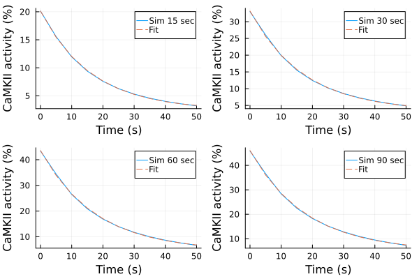

Decay time scales (tau)¶

tau_sim_15 = inv(-fit_sim_15.u.λ[])
tau_sim_30 = inv(-fit_sim_30.u.λ[])
tau_sim_60 = inv(-fit_sim_60.u.λ[])
tau_sim_90 = inv(-fit_sim_90.u.λ[])

println("The time scales for simulations: ")
for (tau, dur) in zip((tau_sim_15, tau_sim_30, tau_sim_60, tau_sim_90), (15, 30, 60, 90))
    println("$dur sec pacing is $(round(tau; digits=2)) seconds.")
end

The time scales for simulations: 
15 sec pacing is 16.3 seconds.
30 sec pacing is 17.07 seconds.
60 sec pacing is 17.6 seconds.
90 sec pacing is 17.98 seconds.

This notebook was generated using Literate.jl.