Electrophysiology - NRVM CaMKII model

Basic CMC model checks

using CSV
using DataFrames
using DiffEqCallbacks
using DifferentialEquations
using Model
using Model: second
using ModelingToolkit
using OrdinaryDiffEqSDIRK
using Plots
using StatsBase: mean
using SteadyStateDiffEq
Plots.default(lw=1.5)

Setup the ODE system¶

Electrical stimulation starts at t=100 sec and ends at t=300 sec.

@time sys = Model.DEFAULT_SYS
tend = 500.0second
@time "Build problem" prob = ODEProblem(sys, [], (0.0, tend))
alg = KenCarp4()

@unpack Istim = sys
stimstart = 100.0second
stimend = 300.0second

  0.000025 seconds (38 allocations: 1.766 KiB)
Build problem: 45.062056 seconds (69.71 M allocations: 3.407 GiB, 5.16% gc time, 99.39% compilation time: 61% of which was recompilation)

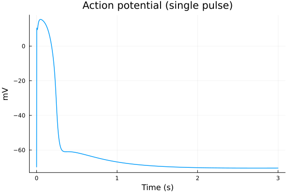
300000.0

Single pulse¶

callback = build_stim_callbacks(Istim, stimstart + 1second; period=10second, starttime=stimstart)
@time sol = solve(prob, alg; callback)

plot(sol, idxs=(sys.t / 1000 - 100, sys.vm), title="Action potential (single pulse)", ylabel="mV", xlabel="Time (s)", label=false, tspan=(100second, 103second))

  5.612538 seconds (14.43 M allocations: 655.997 MiB, 12.06% gc time, 98.35% compilation time)

savefig("single-pulse.pdf")
savefig("single-pulse.png")

"/home/github/actions-runner-2/_work/camkii-cardiomyocyte-model/camkii-cardiomyocyte-model/docs/single-pulse.png"

plot(sol, idxs=(sys.t / 1000 - 100, sys.Cai_mean), tspan=(100second, 103second), title="Calcium transient", ylabel="Conc. (μM)", xlabel="Time (s)", label="Avg Ca")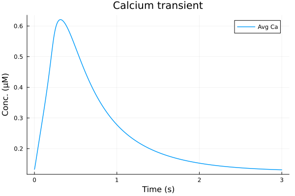

savefig("single-calcium-transient.pdf")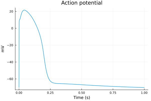
savefig("calcium-transient.png")

"/home/github/actions-runner-2/_work/camkii-cardiomyocyte-model/camkii-cardiomyocyte-model/docs/calcium-transient.png"

1Hz pacing¶

callback = build_stim_callbacks(Istim, stimend; period=1second, starttime=stimstart)
@time sol = solve(prob, alg; callback)
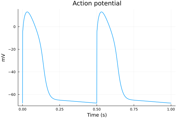
plot(sol, idxs=(sys.t / 1000 - 299, sys.vm), title="Action potential", tspan=(299second, 300second), ylabel="mV", xlabel="Time (s)", label=false)

  2.003087 seconds (98.34 k allocations: 23.049 MiB)

plot(sol, idxs=(sys.t / 1000 - 299, [sys.IK1, sys.Ito, sys.IKs, sys.IKr, sys.If]), tspan=(299second, 300second), ylabel="μA/μF", xlabel="Time (s)", label=["IK1" "Ito" "IKs" "IKr" "If"])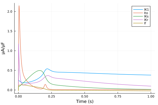

plot(sol, idxs=(sys.t / 1000 - 299, [sys.ICaL, sys.INaCa, sys.ICaT, sys.ICab]), tspan=(299second, 300second), ylabel="μA/μF", xlabel="Time (s)", label=["ICaL" "INaCa" "ICaT" "ICab"])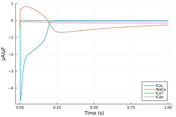

plot(sol, idxs=(sys.t / 1000 - 299, [sys.Cai_sub_SR, sys.Cai_sub_SL, sys.Cai_mean]), tspan=(299second, 300second), title="Calcium transient", ylabel="μM", xlabel="Time (s)", label=["CaSR" "CaSL" "CaAvg"])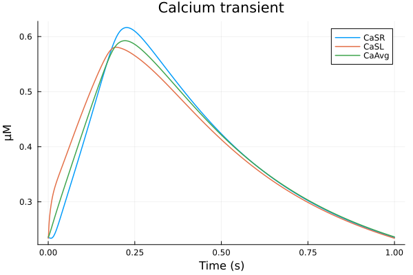

3D surface plot¶

xx = 1:44
yy = range(299second, 300second, length=100)
zz = [sol(t, idxs=sys.Cai[u]) for t in yy, u in xx]

surface(xx, (yy .- 299second) ./ 1000, zz, colorbar=:none, yguide="(sec.)", zguide="Ca Conc. (μM)", xticks=false, size=(600, 600))
annotate!(3, 0, 0.65, "Ca (SL)")
annotate!(41, 0.25, 0.58, "Ca (SR)")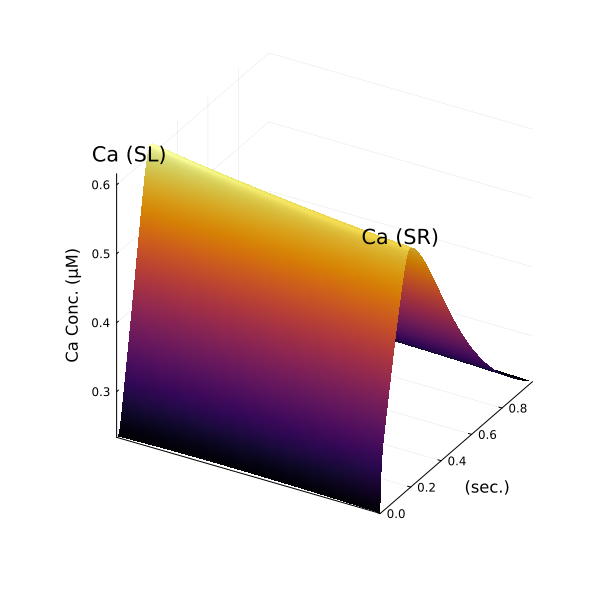

savefig("3d-surface.pdf")
savefig("3d-surface.png")

"/home/github/actions-runner-2/_work/camkii-cardiomyocyte-model/camkii-cardiomyocyte-model/docs/3d-surface.png"

Mean calcium¶

xx = 1:44
yy = [sol(299.22second, idxs=sys.Cai[u]) for u in xx]
avg = mean(yy)

plot(xx, yy, label="Cai", ylabel="Ca Conc. (μM)", xlabel="Compartment (SL to SR)", legend=:topright)
hline!([avg], linestyle=:dash, label="Avg Cai")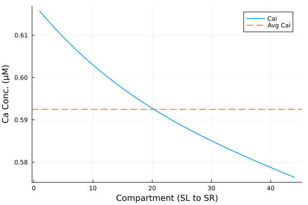

savefig("cai-spatial.pdf")
savefig("cai-spatial.png")

"/home/github/actions-runner-2/_work/camkii-cardiomyocyte-model/camkii-cardiomyocyte-model/docs/cai-spatial.png"

Comparing 1 and 2 Hz pacing¶

callback = build_stim_callbacks(Istim, stimend; period=0.5second, starttime=stimstart)
@time sol2 = solve(prob, alg; callback)

plot(sol2, idxs=(sys.t / 1000 - 299, sys.vm), title="Action potential", tspan=(299second, 300second), ylabel="mV", xlabel="Time (s)", label=false)

  3.507273 seconds (161.21 k allocations: 38.190 MiB)

plot(sol2, idxs=(sys.t / 1000 - 299, [sys.Cai_sub_SR, sys.Cai_sub_SL, sys.Cai_mean]), tspan=(299second, 300second), title="Calcium transient", ylabel="Concentration (μM)", xlabel="Time (s)", label=["CaSSR" "CaSL" "CaAvg"])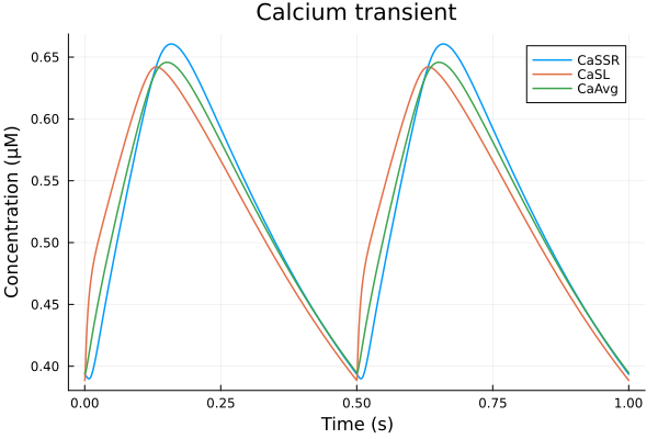

idxs = (sys.t / 1000 - 299, sys.vm)
plot(sol, idxs=idxs, title="Action potential", lab="1Hz", tspan=(299second, 300second))
plot!(sol2, idxs=idxs, lab="2Hz", tspan=(299second, 300second), xlabel="Time (s)", ylabel="Voltage (mV)")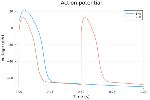

savefig("bcl-ap.pdf")
savefig("bcl-ap.png")

"/home/github/actions-runner-2/_work/camkii-cardiomyocyte-model/camkii-cardiomyocyte-model/docs/bcl-ap.png"

idxs = (sys.t / 1000 - 299, sys.Cai_mean)
plot(sol, idxs=idxs, title="Calcium transient", lab="1Hz", tspan=(299second, 300second))
plot!(sol2, idxs=idxs, lab="2Hz", tspan=(299second, 300second), xlabel="Time (s)", ylabel="Concentration (μM)")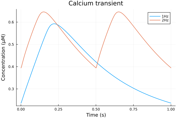

savefig("bcl-cat.pdf")
savefig("bcl-cat.png")

"/home/github/actions-runner-2/_work/camkii-cardiomyocyte-model/camkii-cardiomyocyte-model/docs/bcl-cat.png"

This notebook was generated using Literate.jl.