using Model
using Model: second, μM
import Dates
using CSV
using CurveFit
using DataFrames
using DiffEqCallbacks
using DifferentialEquations
using ModelingToolkit
using OrdinaryDiffEqSDIRK
using Plots
using StatsPlots
Plots.default(lw=1.5)
Setup model
@time "Build system" sys = Model.DEFAULT_SYS
@unpack Istim = sys
tend = 205second
stimstart = 30second
stimend = 120second
newkox_CaMK = inv(45second) / 50μM
@time "Build problem" prob = ODEProblem(sys, [sys.kox_CaMK => inv(45second) / 50μM], tend)
callback = build_stim_callbacks(Istim, stimend; period=1second, starttime=stimstart)
alg = KenCarp4()
Build system: 0.000036 seconds (58 allocations: 2.656 KiB)
Build problem: 91.447819 seconds (162.78 M allocations: 7.940 GiB, 4.31% gc time, 99.77% compilation time: 12% of which was recompilation)
KenCarp4(; linsolve = nothing, nlsolve = OrdinaryDiffEqNonlinearSolve.NLNewton{Rational{Int64}, Rational{Int64}, Rational{Int64}, Nothing}(1//100, 10, 1//5, 1//5, false, true, nothing), smooth_est = true, extrapolant = linear, step_limiter! = trivial_limiter!, autodiff = ADTypes.AutoForwardDiff(), concrete_jac = nothing,)Comparisons
ROS (H2O2) 0uM vs 50uM vs 200uM
@time "Solve problem" sol = solve(prob, alg; callback)

prob2 = remake(prob, p=[sys.ROS => 50μM])
@time "Solve problem" sol2 = solve(prob2, alg; callback)

prob3 = remake(prob, p=[sys.ROS => 200μM])
@time "Solve problem" sol3 = solve(prob3, alg; callback);
Solve problem: 7.747787 seconds (15.69 M allocations: 722.559 MiB, 3.25% gc time, 85.02% compilation time)
Solve problem: 0.850151 seconds (49.48 k allocations: 10.777 MiB)
Solve problem: 0.857379 seconds (49.41 k allocations: 10.751 MiB)
Comparisons
i = (sys.t / 1000, sys.CaMKAct)
plot(sol, idxs=i, lab="ROS (-)", color=:blue)
plot!(sol2, idxs=i, lab="ROS 50uM", color=:red)
plot!(sol3, idxs=i, lab="ROS 200uM", color=:green)
plot!(xlabel="Time (s)", ylabel="Active CaMKII fraction", title="Simulation")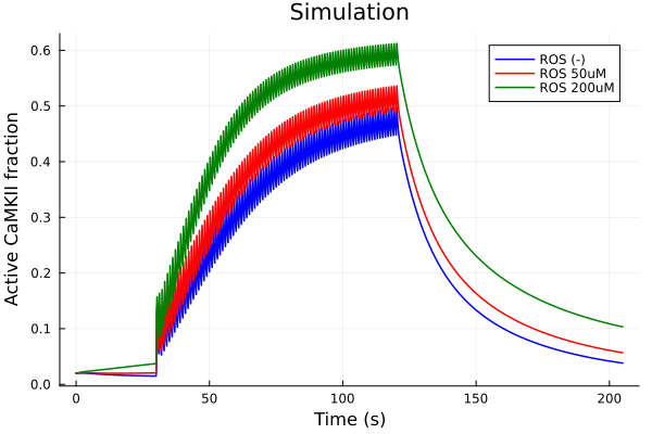
savefig("ros-camkii.pdf")
savefig("ros-camkii.png")"/home/github/actions-runner-2/_work/camkii-cardiomyocyte-model/camkii-cardiomyocyte-model/docs/ros-camkii.png"Oxidized and autophosphorylated fraction
iox = (sys.t / 1000, (sys.CaMKBOX + sys.CaMKPOX + sys.CaMKAOX + sys.CaMKOX))
plot(sol, idxs=iox, lab="ROS (-), OX", color=:blue)
plot!(sol2, idxs=iox, lab="ROS 50uM, OX", color=:red)
plot!(sol3, idxs=iox, lab="ROS 200uM, OX", color=:green)
iphos = (sys.t / 1000, (sys.CaMKP + sys.CaMKA + sys.CaMKA2))
plot!(sol, idxs=iphos, lab="ROS (-), phos", color=:blue, linestyle=:dash)
plot!(sol2, idxs=iphos, lab="ROS 50uM, phos", color=:red, linestyle=:dash)
plot!(sol3, idxs=iphos, lab="ROS 200uM, phos", color=:green, linestyle=:dash)
plot!(xlabel="Time (s)", ylabel="Active CaMKII fraction", title="Simulation")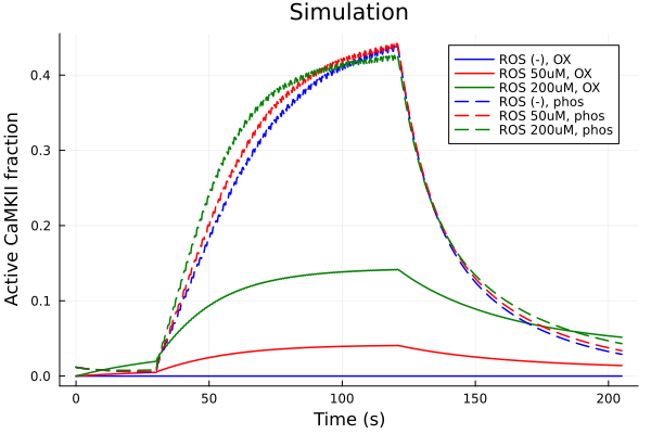
savefig("ros-camkiiox-pox.pdf")
savefig("ros-camkiiox-pox.png")"/home/github/actions-runner-2/_work/camkii-cardiomyocyte-model/camkii-cardiomyocyte-model/docs/ros-camkiiox-pox.png"Proportions for oxidized and autophosphorylated fractions in active CaMKII Using StatsPlots for grouped bar plot at the end of the stimulation period (120 seconds)
timepoint = 120second
pidx = (sys.CaMKP + sys.CaMKA + sys.CaMKA2) / sys.CaMKAct
oidx = (sys.CaMKBOX + sys.CaMKPOX + sys.CaMKAOX + sys.CaMKOX) / sys.CaMKAct
pvals = [s(timepoint, idxs=pidx) for s in (sol, sol2, sol3)]
ovals = [s(timepoint, idxs=oidx) for s in (sol, sol2, sol3)]
groupedbar(["0uM", "50uM", "200uM"], [pvals ovals], bar_position=:stack, label=["Phosphorylated" "Oxidized"], color=[:blue :red :green], title="Simulations", ylabel="Fraction of active CaMKII", xlabel="ROS concentration", legend=:topleft)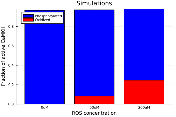
savefig("ros-camkii-groupbar.pdf")
savefig("ros-camkii-groupbar.png")"/home/github/actions-runner-2/_work/camkii-cardiomyocyte-model/camkii-cardiomyocyte-model/docs/ros-camkii-groupbar.png"Experimental data
chemicaldf = CSV.read(joinpath(@__DIR__, "data/CaMKAR-chemical.csv"), DataFrame)
ts = Dates.value.(chemicaldf[!, "Time"]) ./ 10^9
ctl = chemicaldf[!, "Ctrl Mean"]
ctl_error = chemicaldf[!, "Ctrl SD"] ./ sqrt.(chemicaldf[!, "Ctrl N"])
42-element Vector{Float64}:
0.02305850621757014
0.023225557529411765
0.023536003837902393
0.022995786588235295
0.023056161133316953
0.02236794743822152
0.02448575734900888
0.02631837493460871
0.029628792824062226
0.0306227531696316
⋮
0.02665056333747046
0.02525893438851731
0.024749347823716496
0.024158682609370527
0.023572491294117648
0.0240760416039372
0.023230166
0.023759599761907887
0.02369791084482974ros50 = chemicaldf[!, "H2O2 50uM Mean"]
ros50_error = chemicaldf[!, "H2O2 50uM SD"] ./ sqrt.(chemicaldf[!, "H2O2 50uM N"])
ros200 = chemicaldf[!, "H2O2 200uM Mean"]
ros200_error = chemicaldf[!, "H2O2 200uM SD"] ./ sqrt.(chemicaldf[!, "H2O2 200uM N"])42-element Vector{Float64}:
0.01579193843196981
0.015098907892605207
0.01579878654371588
0.015408311367567479
0.01575464714359121
0.015563615686070896
0.015839325542753135
0.01815890968670797
0.022420341690296358
0.026401360928455686
⋮
0.01970504059747541
0.018928610243134615
0.018308801083333333
0.017872510075561544
0.017135324764712814
0.016622042234321177
0.01699837223508933
0.01644948545788867
0.016236308371972322plot(ts, ctl, yerr=ctl_error, lab="Control", color=:blue, markerstrokecolor=:blue)
plot!(ts, ros50, yerr=ros50_error, lab="H2O2 50uM", color=:red, markerstrokecolor=:red)
plot!(ts, ros200, yerr=ros200_error, lab="H2O2 200uM", color=:green, markerstrokecolor=:green)
plot!(xlabel="Time (s)", ylabel="CaMKII activity (A.U.)", title="Experiment")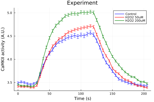
savefig("ros-exp.pdf")
savefig("ros-exp.png")"/home/github/actions-runner-2/_work/camkii-cardiomyocyte-model/camkii-cardiomyocyte-model/docs/ros-exp.png"Decay kinectics
Fit against an exponential decay model.
decay_model(p, x) = @. p[1] * exp(-x / p[2]) + p[3]
Data from experiments (starts from 120 seconds till the end of the experiment).
xdata = collect(range(0.0, step=5.0, length=18))
ydata_ctl = ctl[25:end]
ydata_50 = ros50[25:end]
ydata_200 = ros200[25:end]
ydata_ctl_sim = sol(stimend:5second:tend, idxs=sys.CaMKAct * 100).u
ydata_01_sim = sol2(stimend:5second:tend, idxs=sys.CaMKAct * 100).u
ydata_05_sim = sol3(stimend:5second:tend, idxs=sys.CaMKAct * 100).u
18-element Vector{Float64}:
57.374809641211264
47.76488114828549
39.46360946227911
33.55242722772532
29.162712697344517
25.774771451310592
23.07345404789291
20.862213572745038
19.0140735025373
17.444253203714776
16.09410880980939
14.922061479552799
13.897394265671501
12.996774488045485
12.202035317000458
11.498564062406597
10.874470829650267
10.319851728208338Fit data to an exponential decay model
fit_ctl = solve(CurveFitProblem(xdata, ydata_ctl), ExpSumFitAlgorithm(n=1, withconst=true))
fit_50 = solve(CurveFitProblem(xdata, ydata_50), ExpSumFitAlgorithm(n=1, withconst=true))
fit_200 = solve(CurveFitProblem(xdata, ydata_200), ExpSumFitAlgorithm(n=1, withconst=true))
fit_ctl_sim = solve(CurveFitProblem(xdata, ydata_ctl_sim), ExpSumFitAlgorithm(n=1, withconst=true))
fit_01_sim = solve(CurveFitProblem(xdata, ydata_01_sim), ExpSumFitAlgorithm(n=1, withconst=true))
fit_05_sim = solve(CurveFitProblem(xdata, ydata_05_sim), ExpSumFitAlgorithm(n=1, withconst=true))
retcode: Success
alg: ExpSumFitAlgorithm
residuals mean: 2.7632217501781674e-15
u: [9.901057209717385, 46.60926637340695, -0.0425179354576926]Calculate time scales (tau) from fit parameters
tau_exp_ctl = inv(-fit_ctl.u.λ[])
tau_exp_50 = inv(-fit_50.u.λ[])
tau_exp_200 = inv(-fit_200.u.λ[])
tau_sim_ctl = inv(-fit_ctl_sim.u.λ[])
tau_sim_01 = inv(-fit_01_sim.u.λ[])
tau_sim_05 = inv(-fit_05_sim.u.λ[])

println("The time scales for experiments: ")
for (tau, freq) in zip((tau_exp_ctl, tau_exp_50, tau_exp_200), (0, 50, 200))
    println("$freq uM ROS is $(round(tau; digits=2)) seconds.")
end

println("\nThe time scales for simulations: ")
for (tau, freq) in zip((tau_sim_ctl, tau_sim_01, tau_sim_05), (0, 50, 200))
    println("$freq uM ROS is $(round(tau; digits=2)) seconds.")
end
The time scales for experiments:
0 uM ROS is 25.82 seconds.
50 uM ROS is 31.79 seconds.
200 uM ROS is 37.46 seconds.
The time scales for simulations:
0 uM ROS is 20.51 seconds.
50 uM ROS is 21.5 seconds.
200 uM ROS is 23.52 seconds.
This notebook was generated using Literate.jl.