Pacing frequency - NRVM CaMKII model

1Hz vs 2Hz pacing

using ModelingToolkit
using OrdinaryDiffEq, SteadyStateDiffEq, DiffEqCallbacks
using Plots
using CSV
using DataFrames
using CurveFit
using Model
using Model: second
Plots.default(lw=1.5)

Experiments¶

freqdf = CSV.read(joinpath(@__DIR__, "data/CaMKAR-freq.csv"), DataFrame)
ts = 0:5:205
onehz = freqdf[!, "1Hz (Mean)"]
onehz_error = freqdf[!, "1Hz (SD)"] ./ sqrt.(freqdf[!, "1Hz (N)"])
twohz = freqdf[!, "2Hz (Mean)"]
twohz_error = freqdf[!, "2Hz (SD)"] ./ sqrt.(freqdf[!, "2Hz (N)"])

plot(ts, onehz, yerr=onehz_error, lab="1 Hz", color=:blue, markerstrokecolor=:blue)
plot!(ts, twohz, yerr=twohz_error, lab="2 Hz", color=:red, markerstrokecolor=:red)
plot!(title="Experiment", xlabel="Time (s)", ylabel="CaMKII activity (AU)")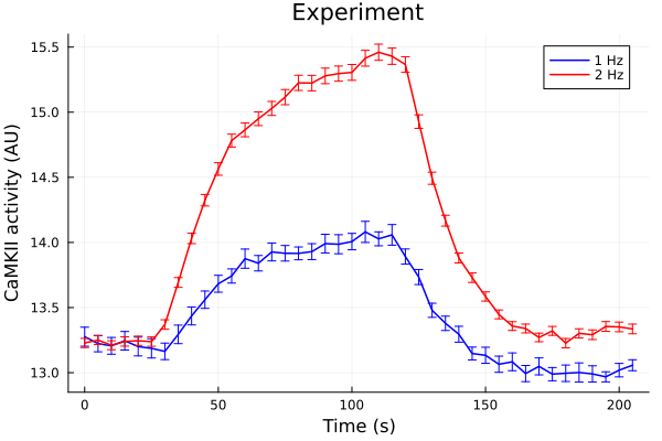

savefig("pacing-frequency-exp.pdf")

"/home/runner/work/camkii-cardiomyocyte-model/camkii-cardiomyocyte-model/docs/pacing-frequency-exp.pdf"

Simulations¶

@time "Build system" sys = Model.DEFAULT_SYS
tend = 205.0second
@time "Build problem" prob = ODEProblem(sys, [], tend)

Build system: 0.000003 seconds
Build problem: 41.285534 seconds (49.74 M allocations: 3.437 GiB, 3.47% gc time, 99.52% compilation time: 39% of which was recompilation)

ODEProblem with uType Vector{Float64} and tType Float64. In-place: true
Initialization status: FULLY_DETERMINED
Non-trivial mass matrix: false
timespan: (0.0, 205000.0)
u0: 75-element Vector{Float64}:
    830.0
    830.0
      0.0026
      0.07192
      0.07831
      0.26081
      0.00977
      0.00188
      0.09243
      0.22156
      ⋮
      0.12113
      0.12113
      0.12113
      0.12113
      0.12113
      0.12113
 150952.75035000002
  13838.37602
    -68.79268

@unpack Istim = sys
stimstart = 30.0second
stimend = 120.0second
alg = KenCarp47()

callback = build_stim_callbacks(Istim, stimend; period=1second, starttime=stimstart)
@time "Solve problem" sol1 = solve(prob, alg; callback)

callback2 = build_stim_callbacks(Istim, stimend; period=0.5second, starttime=stimstart)
@time "Solve problem" sol2 = solve(prob, alg; callback=callback2)

idxs = (sys.t / 1000, sys.CaMKAct * 100)
idxs_phos = (sys.t / 1000, (sys.CaMKP + sys.CaMKA + sys.CaMKA2) * 100)
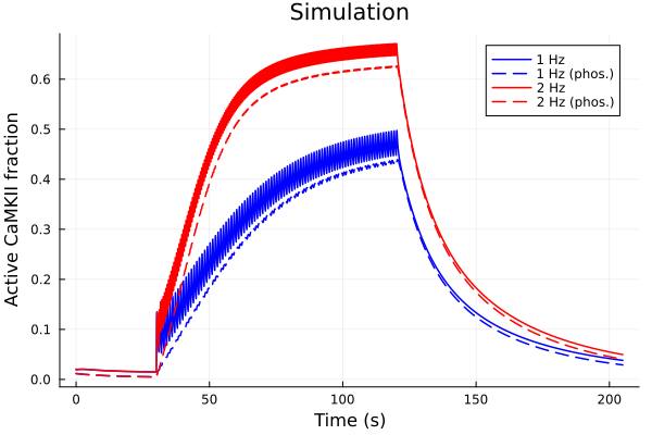
plot(sol1, idxs=idxs, lab="1 Hz", color=:blue)
plot!(sol1, idxs=idxs_phos, lab="1 Hz (phos.)", color=:blue, linestyle=:dash)
plot!(sol2, idxs=idxs, lab="2 Hz", color=:red)
plot!(sol2, idxs=idxs_phos, lab="2 Hz (phos.)", color=:red, linestyle=:dash)
plot!(title="Simulation", xlabel="Time (s)", ylabel="CaMKII activity (%)")

Solve problem: 4.881089 seconds (7.46 M allocations: 701.783 MiB, 3.03% gc time, 77.76% compilation time)
Solve problem: 1.706113 seconds (850.54 k allocations: 354.746 MiB, 1.53% gc time)

savefig("pacing-frequency-sim.pdf")

"/home/runner/work/camkii-cardiomyocyte-model/camkii-cardiomyocyte-model/docs/pacing-frequency-sim.pdf"

Decay rates¶

Fit against an exponential decay model.

decay_model(p, x) = p[1] * exp(-x / p[2]) + p[3]

Data from experiments: record 50 seconds after pacing ends

ts = collect(range(0.0, stop=50.0, step=5.0))
ydata_1hz = onehz[24:34]
ydata_2hz = twohz[24:34]

11-element Vector{Float64}:
 15.42960935
 15.36597804
 14.9277179
 14.49292672
 14.16724572
 13.88090175
 13.72945046
 13.58492818
 13.44736726
 13.35805848
 13.33923508

Simulated data

ysim_1hz = sol1(stimend:5second:stimend+50second; idxs=sys.CaMKAct * 100).u
ysim_2hz = sol2(stimend:5second:stimend+50second; idxs=sys.CaMKAct * 100).u

11-element Vector{Float64}:
 62.30594154582065
 48.251365955092986
 37.31266003345509
 29.667590162331148
 24.21687244765909
 20.20356618969857
 17.149567168417928
 14.754630781381787
 12.828710819127231
 11.247512300011767
  9.928133239576226

Fit data to an exponential decay model

fit_1hz = solve(CurveFitProblem(ts, ydata_1hz), ExpSumFitAlgorithm(n=1, withconst=true))
fit_2hz = solve(CurveFitProblem(ts, ydata_2hz), ExpSumFitAlgorithm(n=1, withconst=true))
fit_1hz_sim = solve(CurveFitProblem(ts, ysim_1hz), ExpSumFitAlgorithm(n=1, withconst=true))
fit_2hz_sim = solve(CurveFitProblem(ts, ysim_2hz), ExpSumFitAlgorithm(n=1, withconst=true))

retcode: Success
alg: ExpSumFitAlgorithm
residuals mean: 3.552713678800501e-15
u: [7.516166658834331, 54.597551715642545, -0.05907841253955547]

Fitting results (experiments)

p1 = plot(ts, ydata_1hz, label="Exp 1 Hz")
plot!(p1, ts, predict(fit_1hz), label="Fit", linestyle=:dash)
p2 = plot(ts, ydata_2hz, label="Exp 2 Hz")
plot!(p2, ts, predict(fit_2hz), label="Fit", linestyle=:dash)
p3 = plot(ts, ysim_1hz, label="Sim 1 Hz")
plot!(p3, ts, predict(fit_1hz_sim), label="Fit", linestyle=:dash)
p4 = plot(ts, ysim_2hz, label="Sim 2 Hz")
plot!(p4, ts, predict(fit_2hz_sim), label="Fit", linestyle=:dash)
plot(p1, p2, p3, p4, layout=(2,2), xlabel="Time (s)", ylabel="CaMKII activity (AU)")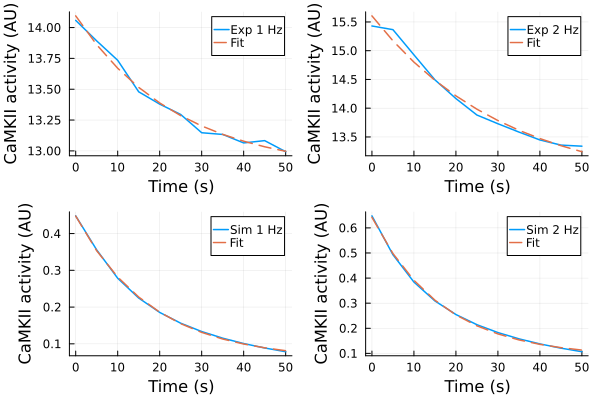

Decay time scales (tau) from fit parameters

tau_exp_1hz = inv(-fit_1hz.u.λ[])
tau_exp_2hz = inv(-fit_2hz.u.λ[])
tau_sim_1hz = inv(-fit_1hz_sim.u.λ[])
tau_sim_2hz = inv(-fit_2hz_sim.u.λ[])

println("The time scales for experiments: ")
for (tau, freq) in zip((tau_exp_1hz, tau_exp_2hz), (1, 2))
    println("$freq Hz pacing is $(round(tau; digits=2)) seconds.")
end
println("The time scales for simulations: ")
for (tau, freq) in zip((tau_sim_1hz, tau_sim_2hz), (1, 2))
    println("$freq Hz pacing is $(round(tau; digits=2)) seconds.")
end

The time scales for experiments: 
1 Hz pacing is 24.31 seconds.
2 Hz pacing is 31.82 seconds.
The time scales for simulations: 
1 Hz pacing is 18.08 seconds.
2 Hz pacing is 16.93 seconds.

This notebook was generated using Literate.jl.