b1AR system simplification - NRVM CaMKII model

Fitting sensitivity of b1AR system to ISO.

using Model
using Model: Hz, hil, hilr, second, μM

using CurveFit
using DiffEqCallbacks
using DifferentialEquations
using ModelingToolkit
using OrdinaryDiffEqSDIRK
using Plots
using SteadyStateDiffEq
Plots.default(lw=1.5)

Setup b1AR system¶

@parameters ATP = 5000μM ISO = 0μM
@time "Build system" sys = Model.get_bar_sys(ATP, ISO) |> mtkcompile
@time "Build problem" prob = SteadyStateProblem(sys, [])

alg = DynamicSS(KenCarp4())
@time "Solve problem" sol = solve(prob, alg; abstol=1e-9, reltol=1e-9)

Build system: 57.929375 seconds (72.36 M allocations: 3.523 GiB, 2.54% gc time, 99.94% compilation time: 33% of which was recompilation)
Build problem: 19.694030 seconds (55.05 M allocations: 2.757 GiB, 5.57% gc time, 99.41% compilation time: 19% of which was recompilation)
Solve problem: 3.937183 seconds (9.45 M allocations: 474.815 MiB, 1.38% gc time, 99.59% compilation time)

retcode: Success
u: 27-element Vector{Float64}:
 0.027718161383497624
 0.010978639935515684
 0.006295471962435581
 0.005515872061732562
 4.449170371402564
 5.432765220910506
 8.127509227640667
 0.05167159021772034
 0.06163645372117289
 0.036126889458918836
 ⋮
 0.002234002469315477
 0.0014298729000213404
 0.0005917175909915705
 1.516109097808491e-6
 0.0006214228121296868
 0.008288863258287149
 0.00048593702847026665
 1.5286323837495727e-10
 3.121934781705491e-12

@unpack cAMP, fracPKACI, fracPKACII, fracPP1, fracPLBp, fracPLMp, TnI_PKAp, LCCa_PKAp, LCCb_PKAp, IKUR_PKAp, RyR_PKAp = sys
tracked_states = [cAMP, fracPKACI, fracPKACII, fracPP1, fracPLBp, fracPLMp, TnI_PKAp, LCCa_PKAp, LCCb_PKAp, IKUR_PKAp, RyR_PKAp]
stimap = Dict(k=>i for (i, k) in enumerate(tracked_states))

@time "Extract tracked states" sol[tracked_states]

Extract tracked states: 1.025974 seconds (1.25 M allocations: 63.202 MiB, 99.79% compilation time)

11-element Vector{Float64}:
 0.290372796633918
 0.07297414401912693
 0.1836654167735595
 0.9419420334632356
 0.07667461535510063
 0.11318260876896886
 0.06355957673432235
 0.2206348824693025
 0.25181887849742324
 0.43914559742062736
 0.20531971395183424

Ensemble simulations¶

Log scale for ISO concentration.

iso = exp10.(range(log10(1e-4μM), log10(1μM), length=501))

@time "Solve problems" sim = map(iso) do i
    newprob = remake(prob, p=[ISO => i])
    solve(newprob, alg; abstol=1e-9, reltol=1e-9)[tracked_states]
end

yymat = reduce(hcat, sim)'

Solve problems: 28.131783 seconds (114.10 M allocations: 5.794 GiB, 3.31% gc time, 31.33% compilation time: 3% of which was recompilation)

501×11 adjoint(::Matrix{Float64}) with eltype Float64:
 0.295127  0.074457   0.187039  0.941176  …  0.255326  0.443686  0.208476
 0.295215  0.0744844  0.187101  0.941162     0.255391  0.443769  0.208535
 0.295303  0.074512   0.187164  0.941148     0.255455  0.443853  0.208593
 0.295395  0.0745407  0.187229  0.941133     0.255523  0.44394   0.208654
 0.295487  0.0745693  0.187294  0.941119     0.25559   0.444027  0.208714
 0.295582  0.074599   0.187362  0.941103  …  0.25566   0.444116  0.208777
 0.295679  0.0746289  0.18743   0.941088     0.25573   0.444207  0.20884
 0.295776  0.0746591  0.187498  0.941073     0.255801  0.444298  0.208904
 0.295876  0.0746903  0.187569  0.941057     0.255874  0.444393  0.20897
 0.295977  0.0747218  0.18764   0.941041     0.255948  0.444488  0.209037
 ⋮                                        ⋱                      ⋮
 1.13236   0.270231   0.524879  0.893        0.495933  0.693674  0.443452
 1.13269   0.270285   0.524947  0.892993     0.495967  0.693702  0.443487
 1.63512   0.341451   0.604672  0.886288     0.532098  0.72317   0.481555
 1.63576   0.341527   0.604749  0.886282  …  0.53213   0.723196  0.48159
 1.13372   0.270457   0.525163  0.892974     0.496072  0.69379   0.443596
 1.13407   0.270516   0.525237  0.892967     0.496108  0.69382   0.443634
 1.13441   0.270574   0.525309  0.892961     0.496143  0.693849  0.443671
 1.13471   0.270623   0.525371  0.892955     0.496173  0.693875  0.443703
 1.13504   0.270679   0.525441  0.892949  …  0.496207  0.693903  0.443738

xopts = (xlims=(iso[begin], iso[end]), minorgrid=true, xscale=:log10, xlabel="ISO (μM)",)
plot(iso, yymat[:, stimap[cAMP]]; lab="cAMP", ylabel="Conc. (μM)", legend=:topleft, xopts...)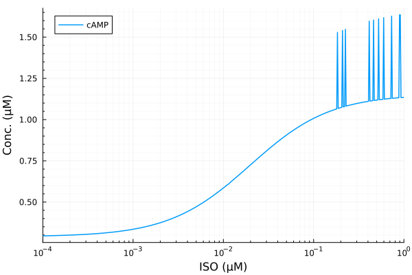

plot(iso, yymat[:, stimap[fracPKACI]]; lab="PKACI", ylabel="Activation fraction")
plot!(iso, yymat[:, stimap[fracPKACII]], lab="PKACII")
plot!(iso, yymat[:, stimap[fracPP1]], lab="PP1", legend=:topleft; xopts...)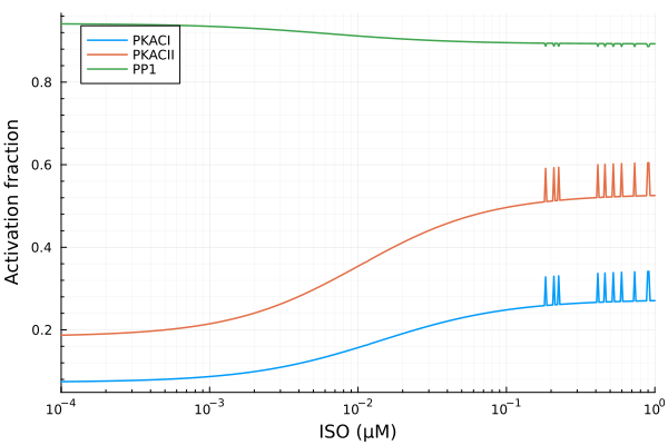

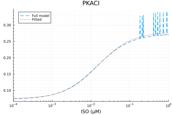
PKACI activity¶

pkaci_model(p, x) = @. p[1] * hil(x, p[2]) + p[3]
xdata = iso
ydata = yymat[:, stimap[fracPKACI]]
p0 = [0.3, 0.01μM, 0.08]
prob = NonlinearCurveFitProblem(pkaci_model, p0, xdata, ydata)
@time "Fit PKACI" fit_pkac1 = solve(prob)

println("PKACI")
println("Basal activity: ", fit_pkac1.u[3])
println("Activated activity: ", fit_pkac1.u[1])
println("Michaelis constant: ", fit_pkac1.u[2], " μM")
println("RMSE: ", mse(fit_pkac1) |> sqrt)

plot(xdata, [ydata predict(fit_pkac1)], lab=["Full model" "Fitted"], line=[:dash :dot], title="PKACI", legend=:topleft; xopts...)

Fit PKACI: 3.457474 seconds (7.77 M allocations: 390.913 MiB, 1.96% gc time, 99.92% compilation time)
PKACI
Basal activity: 0.07422772672567302
Activated activity: 0.20505258156689657
Michaelis constant: 0.01524715576250627 μM
RMSE: 0.00960056893192453

savefig("pkaci_fit.pdf")

"/home/github/actions-runner-2/_work/camkii-cardiomyocyte-model/camkii-cardiomyocyte-model/docs/fits/pkaci_fit.pdf"

plot(xdata, residuals(fit_pkac1) ./ ydata .* 100; title="PKACI error (%)", lab=false, xopts...)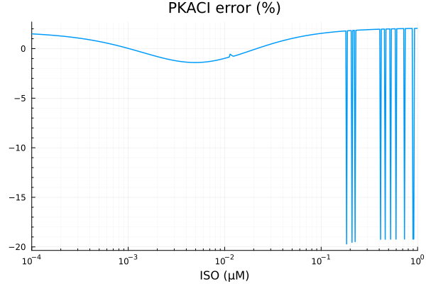

PKACII activity¶

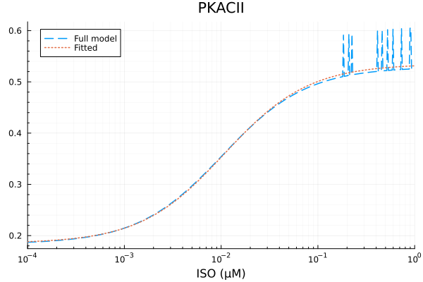
pkacii_model(p, x) = @. p[1] * hil(x, p[2]) + p[3]
xdata = iso
ydata = yymat[:, stimap[fracPKACII]]
p0 = [0.4, 0.01μM, 0.2]
prob = NonlinearCurveFitProblem(pkacii_model, p0, xdata, ydata)
@time fit_pkac2 = solve(prob)

println("PKACII")
println("Basal activity: ", fit_pkac2.u[3])
println("Activated activity: ", fit_pkac2.u[1])
println("Michaelis constant: ", fit_pkac2.u[2], " μM")
println("RMSE: ", mse(fit_pkac2) |> sqrt)

plot(xdata, [ydata predict(fit_pkac2)], lab=["Full model" "Fitted"], line=[:dash :dot], title="PKACII", legend=:topleft; xopts...)

  2.992711 seconds (6.97 M allocations: 350.210 MiB, 2.16% gc time, 99.92% compilation time)
PKACII
Basal activity: 0.18499467578709322
Activated activity: 0.3500460127291659
Michaelis constant: 0.010862206778770832 μM
RMSE: 0.010927086626045626

savefig("pkacii_fit.pdf")

"/home/github/actions-runner-2/_work/camkii-cardiomyocyte-model/camkii-cardiomyocyte-model/docs/fits/pkacii_fit.pdf"

plot(xdata, residuals(fit_pkac2) ./ ydata .* 100; title="PKACII error (%)", lab=false, xopts...)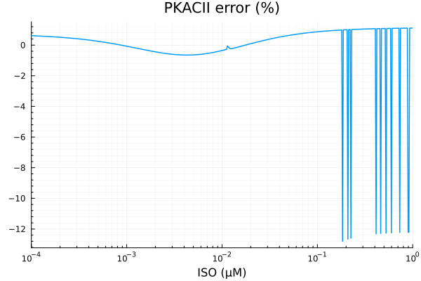

PP1 activity¶

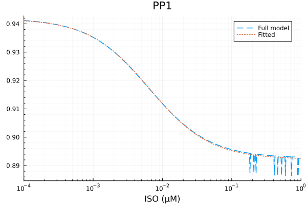
pp1_model(p, x) = @. p[1] * hil(p[2], x) + p[3]
xdata = iso
ydata = yymat[:, stimap[fracPP1]]
p0 = [0.1, 3e-3μM, 0.8]
prob = NonlinearCurveFitProblem(pp1_model, p0, xdata, ydata)
@time fit_pp1 = solve(prob)

println("PP1")
println("Repressible activity: ", fit_pp1.u[1])
println("Minimal activity: ", fit_pp1.u[3])
println("Repressive Michaelis constant: ", fit_pp1.u[2], " μM")
println("RMSE: ", mse(fit_pp1) |> sqrt)

plot(xdata, [ydata predict(fit_pp1)], lab=["Full model" "Fitted"], line=[:dash :dot], title="PP1", legend=:topright; xopts...)

  2.945767 seconds (7.24 M allocations: 363.596 MiB, 1.94% gc time, 99.92% compilation time)
PP1
Repressible activity: 0.04958803301175277
Minimal activity: 0.8922211841997849
Repressive Michaelis constant: 0.006572675578685927 μM
RMSE: 0.0009347259241307221

savefig("pp1_fit.pdf")

"/home/github/actions-runner-2/_work/camkii-cardiomyocyte-model/camkii-cardiomyocyte-model/docs/fits/pp1_fit.pdf"

plot(xdata, residuals(fit_pp1) ./ ydata .* 100; title="PP1 error (%)", lab=false, xopts...)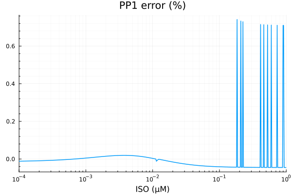

PLBp¶

xdata = iso
ydata = yymat[:, stimap[fracPLBp]]
plot(xdata, ydata, title="PLBp fraction", lab=false; xopts...)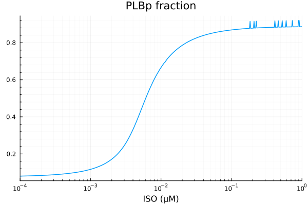

plb_model(p, x) = @. p[1] * hil(x, p[2], p[3]) + p[4]
p0 = [0.8, 1e-2μM, 1.0, 0.1]
prob = NonlinearCurveFitProblem(plb_model, p0, xdata, ydata)
@time fit_plb = solve(prob)

println("PLBp")
println("Basal activity: ", fit_plb.u[4])
println("Activated activity: ", fit_plb.u[1])
println("Michaelis constant: ", fit_plb.u[2], " μM")
println("Hill coefficient: ", fit_plb.u[3])
println("RMSE: ", mse(fit_plb) |> sqrt)

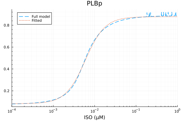
plot(xdata, [ydata predict(fit_plb)], lab=["Full model" "Fitted"], line=[:dash :dot], title="PLBp", legend=:topleft; xopts...)

  3.028253 seconds (7.32 M allocations: 368.952 MiB, 2.07% gc time, 99.61% compilation time)
PLBp
Basal activity: 0.08259325344228947
Activated activity: 0.795066554552995
Michaelis constant: 0.00596246819893431 μM
Hill coefficient: 1.823868532725476
RMSE: 0.010277225658558342

savefig("plbp_fit.pdf")

"/home/github/actions-runner-2/_work/camkii-cardiomyocyte-model/camkii-cardiomyocyte-model/docs/fits/plbp_fit.pdf"

plot(xdata, residuals(fit_plb) ./ ydata .* 100; title="PLBp error (%)", lab=false, xopts...)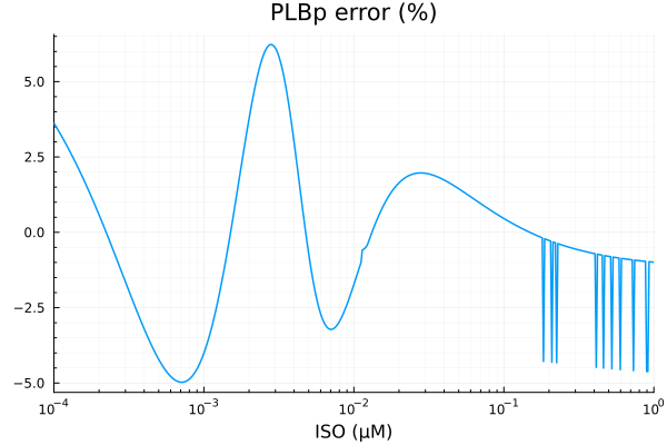

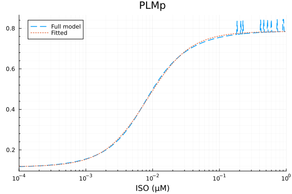
PLMp¶

xdata = iso
ydata = yymat[:, stimap[fracPLMp]]
plot(xdata, ydata, title="PLMp fraction", lab=false; xopts...)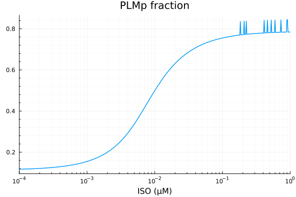

plm_model(p, x) = @. p[1] * hil(x, p[2], p[3]) + p[4]
p0 = [0.8, 1e-2μM, 1.0, 0.1]
prob = NonlinearCurveFitProblem(plm_model, p0, xdata, ydata)
@time fit_plm = solve(prob)

println("PLMp")
println("Basal activity: ", fit_plm.u[4])
println("Activated activity: ", fit_plm.u[1])
println("Michaelis constant: ", fit_plm.u[2], " μM")
println("Hill coefficient: ", fit_plm.u[3])
println("RMSE: ", mse(fit_plm) |> sqrt)

plot(xdata, [ydata predict(fit_plm)], lab=["Full model" "Fitted"], line=[:dash :dot], title="PLMp", legend=:topleft; xopts...)

  2.997675 seconds (7.05 M allocations: 354.942 MiB, 2.05% gc time, 99.64% compilation time)
PLMp
Basal activity: 0.11672865699214915
Activated activity: 0.6680976660156412
Michaelis constant: 0.008296796037780142 μM
Hill coefficient: 1.3463569091924366
RMSE: 0.009446461962283244

savefig("plmp_fit.pdf")

"/home/github/actions-runner-2/_work/camkii-cardiomyocyte-model/camkii-cardiomyocyte-model/docs/fits/plmp_fit.pdf"

plot(xdata, residuals(fit_plm) ./ ydata .* 100; title="PLMp error (%)", lab=false, xopts...)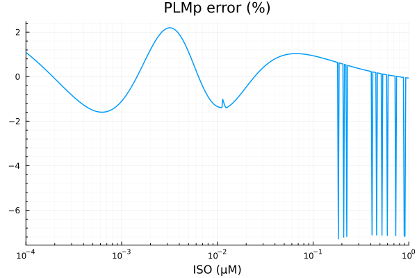

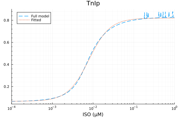
TnIp¶

xdata = iso
ydata = yymat[:, stimap[TnI_PKAp]]
plot(xdata, ydata, title="TnIp fraction", lab=false; xopts...)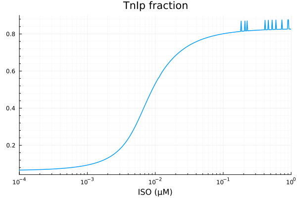

tni_model(p, x) = @. p[1] * hil(x, p[2], p[3]) + p[4]
p0 = [0.8, 1e-2μM, 1.0, 0.1]
lb = [0.1, 1e-9μM, 1.0, 0.0]
prob = NonlinearCurveFitProblem(tni_model, p0, xdata, ydata)
@time fit_tni = solve(prob)

println("TnIp")
println("Basal activity: ", fit_tni.u[4])
println("Activated activity: ", fit_tni.u[1])
println("Michaelis constant: ", fit_tni.u[2], " μM")
println("Hill coefficient: ", fit_tni.u[3])
println("RMSE: ", mse(fit_tni) |> sqrt)

plot(xdata, [ydata predict(fit_tni)], lab=["Full model" "Fitted"], line=[:dash :dot], title="TnIp", legend=:topleft; xopts...)

  3.041665 seconds (7.05 M allocations: 355.068 MiB, 4.89% gc time, 99.63% compilation time)
TnIp
Basal activity: 0.06692214329005741
Activated activity: 0.7527072435918196
Michaelis constant: 0.0079200853867431 μM
Hill coefficient: 1.6753447104293941
RMSE: 0.010986208057286123

savefig("tni_fit.pdf")

"/home/github/actions-runner-2/_work/camkii-cardiomyocyte-model/camkii-cardiomyocyte-model/docs/fits/tni_fit.pdf"

plot(xdata, residuals(fit_tni) ./ ydata .* 100; title="TnIp error (%)", lab=false, xopts...)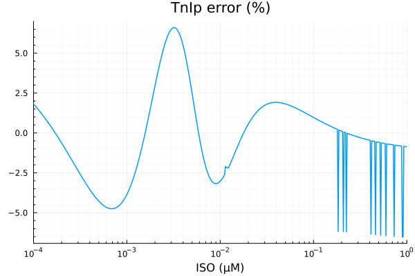

LCCap¶

xdata = iso
ydata = yymat[:, stimap[LCCa_PKAp]]
plot(xdata, ydata, title="LCCap fraction", lab=false; xopts...)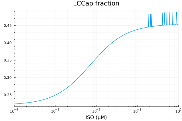

lcc_model(p, x) = @. p[1] * hil(x, p[2]) + p[3]
p0 = [0.8, 1e-2μM, 0.1]
prob = NonlinearCurveFitProblem(lcc_model, p0, xdata, ydata)
@time fit_lcca = solve(prob)

println("LCCap")
println("Basal activity: ", fit_lcca.u[3])
println("Activated activity: ", fit_lcca.u[1])
println("Michaelis constant: ", fit_lcca.u[2], " μM")
println("RMSE: ", mse(fit_lcca) |> sqrt)

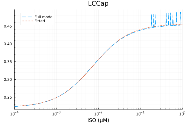
plot(xdata, [ydata predict(fit_lcca)], lab=["Full model" "Fitted"], line=[:dash :dot], title="LCCap", legend=:topleft; xopts...)

  3.355684 seconds (6.97 M allocations: 351.013 MiB, 14.56% gc time, 99.93% compilation time)
LCCap
Basal activity: 0.2213168301495287
Activated activity: 0.2356295423480066
Michaelis constant: 0.0075401946326636516 μM
RMSE: 0.0050019520308986565

savefig("lcca_fit.pdf")

"/home/github/actions-runner-2/_work/camkii-cardiomyocyte-model/camkii-cardiomyocyte-model/docs/fits/lcca_fit.pdf"

plot(xdata, residuals(fit_lcca) ./ ydata .* 100; title="LCCap error (%)", lab=false, xopts...)

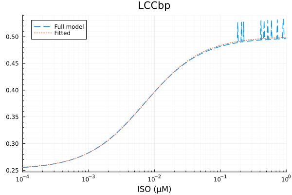
LCCbp¶

xdata = iso
ydata = yymat[:, stimap[LCCb_PKAp]]
plot(xdata, ydata, title="LCCbp fraction", lab=false; xopts...)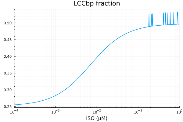

p0 = [0.8, 1e-2μM, 0.1]
lb = [0.1, 1e-9μM, 0.0]
prob = NonlinearCurveFitProblem(lcc_model, p0, xdata, ydata)
@time fit_lccb = solve(prob)

println("LCCbp")
println("Basal activity: ", fit_lccb.u[3])
println("Activated activity: ", fit_lccb.u[1])
println("Michaelis constant: ", fit_lccb.u[2], " μM")
println("RMSE: ", mse(fit_lccb) |> sqrt)

plot(xdata, [ydata predict(fit_lccb)], lab=["Full model" "Fitted"], line=[:dash :dot], title="LCCbp", legend=:topleft; xopts...)

  0.000969 seconds (1.62 k allocations: 2.794 MiB)
LCCbp
Basal activity: 0.2525121186801279
Activated activity: 0.24780603459061848
Michaelis constant: 0.0072127232713688335 μM
RMSE: 0.005022057891599535

savefig("lccbp_fit.pdf")

"/home/github/actions-runner-2/_work/camkii-cardiomyocyte-model/camkii-cardiomyocyte-model/docs/fits/lccbp_fit.pdf"

plot(xdata, residuals(fit_lccb) ./ ydata .* 100; title="LCCbp error (%)", lab=false, xopts...)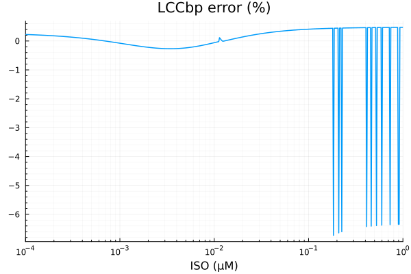

KURp¶

xdata = iso
ydata = yymat[:, stimap[IKUR_PKAp]]
plot(xdata, ydata, title="KURp fraction", lab=false; xopts...)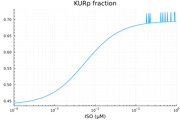

kur_model(p, x) = @. p[1] * hil(x, p[2]) + p[3]
p0 = [0.8, 1e-2μM, 0.1]
lb = [0.1, 1e-9μM, 0.0]
prob = NonlinearCurveFitProblem(kur_model, p0, xdata, ydata)
@time fit_kur = solve(prob)

println("KURp")
println("Basal activity: ", fit_kur.u[3])
println("Activated activity: ", fit_kur.u[1])
println("Michaelis constant: ", fit_kur.u[2], " μM")
println("RMSE: ", mse(fit_kur) |> sqrt)

plot(xdata, [ydata predict(fit_kur)], lab=["Full model" "Fitted"], line=[:dash :dot], title="KURp", legend=:topleft; xopts...)

  2.825441 seconds (6.97 M allocations: 350.330 MiB, 99.91% compilation time)
KURp
Basal activity: 0.4397979902461887
Activated activity: 0.25731764310948285
Michaelis constant: 0.005732486840439236 μM
RMSE: 0.004125437957358825

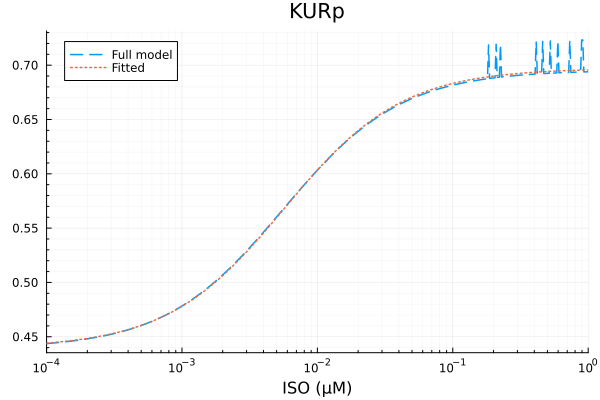
savefig("kurp_fit.pdf")

"/home/github/actions-runner-2/_work/camkii-cardiomyocyte-model/camkii-cardiomyocyte-model/docs/fits/kurp_fit.pdf"

plot(xdata, residuals(fit_kur) ./ ydata .* 100; title="KURp error (%)", lab=false, xopts...)

RyRp¶

xdata = iso
ydata = yymat[:, stimap[RyR_PKAp]]
plot(xdata, ydata, title="RyRp fraction", lab=false; xopts...)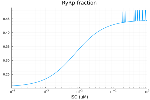

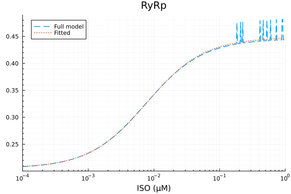
ryr_model(p, x) = @. p[1] * x / (x + p[2]) + p[3]
p0 = [0.3, 1e-2μM, 0.1]
lb = [0.0, 1e-9μM, 0.0]
prob = NonlinearCurveFitProblem(ryr_model, p0, xdata, ydata)
@time fit_ryr = solve(prob)

println("RyRp")
println("Basal activity: ", fit_ryr.u[3])
println("Activated activity: ", fit_ryr.u[1])
println("Michaelis constant: ", fit_ryr.u[2], " μM")
println("RMSE: ", mse(fit_ryr) |> sqrt)

plot(xdata, [ydata predict(fit_ryr)], lab=["Full model" "Fitted"], line=[:dash :dot], title="RyRp", legend=:topleft; xopts...)

  2.866783 seconds (7.46 M allocations: 374.602 MiB, 2.43% gc time, 99.92% compilation time)
RyRp
Basal activity: 0.20591740824163482
Activated activity: 0.24229333603081707
Michaelis constant: 0.0078047893771042 μM
RMSE: 0.005271982807636429

savefig("ryrp_fit.pdf")

"/home/github/actions-runner-2/_work/camkii-cardiomyocyte-model/camkii-cardiomyocyte-model/docs/fits/ryrp_fit.pdf"

plot(xdata, residuals(fit_ryr) ./ ydata .* 100; title="RyRp error (%)", lab=false, xopts...)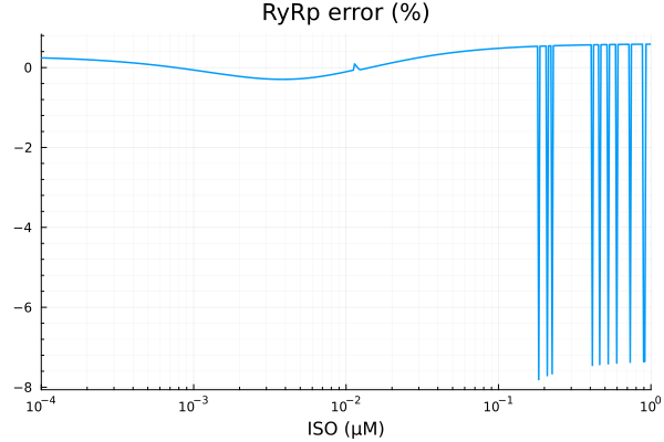

This notebook was generated using Literate.jl.