using Model
using Model: μM, hil, second, Hz
using CurveFit
using DiffEqCallbacks
using DifferentialEquations
using ModelingToolkit
using OrdinaryDiffEqSDIRK
using Plots
using SteadyStateDiffEq
Plots.default(lw=1.5)
CaMKII sensitivity to calcium
Modeling CaM-Cax binding to CaMKII only. No phosphorylation or oxidation reactions.
@parameters Ca = 0μM ROS = 0μM
@time "Build system" sys = Model.get_camkii_sys(; Ca=Ca, ROS=ROS) |> mtkcompile
@time "Build problem" prob = SteadyStateProblem(sys, [sys.k_phosCaM => 0])
Build system: 53.297799 seconds (69.40 M allocations: 3.398 GiB, 3.19% gc time, 99.93% compilation time: 46% of which was recompilation)
Build problem: 20.510291 seconds (54.70 M allocations: 2.743 GiB, 5.27% gc time, 99.78% compilation time: 19% of which was recompilation)
SteadyStateProblem with uType Vector{Float64}. In-place: true
u0: 17-element Vector{Float64}:
 0.0
 0.0
 0.0
 3.3
 0.0
 0.0
 0.01581
 0.010750000000000001
 1.01
 0.62372
 0.00666
 0.0166
 0.39868000000000003
 1.0
 2.0e-5
 0.008577999999999999
 0.08433
Physiological cytosolic calcium levels ranges from 30nM to 10μM.
ca = exp10.(range(log10(0.03μM), log10(10μM), length=1001))
@time "Solve problem" sim = map(ca) do c
    newprob = remake(prob, p=[Ca => c])
    solve(newprob, DynamicSS(KenCarp4()); abstol=1e-8, reltol=1e-8)
end;
Solve problem: 30.261852 seconds (112.72 M allocations: 5.356 GiB, 8.18% gc time, 27.64% compilation time: 22% of which was recompilation)
"""Extract values from ensemble simulations by a symbol"""
extract(sim, k) = map(s -> s[k], sim)Main.var"##288".extractStatus of the CaMKII system across a range of calcium concentrations.
xopts = (xlabel="Ca (μM)", xscale=:log10, minorgrid=true, xlims=(ca[1], ca[end]))
let
    plot(ca, extract(sim, sys.Ca2CaM_C), lab="Ca2CaM_C", ylabel="Conc. (μM)"; xopts...)
    plot!(ca, extract(sim, sys.Ca2CaM_N), lab="Ca2CaM_N")
    plot!(ca, extract(sim, sys.Ca4CaM), lab="Ca4CaM")
    plot!(ca, extract(sim, sys.CaMK), lab="CaMK")
    plot!(ca, extract(sim, sys.CaM0_CaMK), lab="CaM0_CaMK")
    plot!(ca, extract(sim, sys.Ca2CaM_C_CaMK), lab="Ca2CaM_C_CaMK")
    plot!(ca, extract(sim, sys.Ca2CaM_N_CaMK), lab="Ca2CaM_N_CaMK")
    plot!(ca, extract(sim, sys.Ca4CaM_CaMK), lab="Ca4CaM_CaMK", legend=:topleft)
end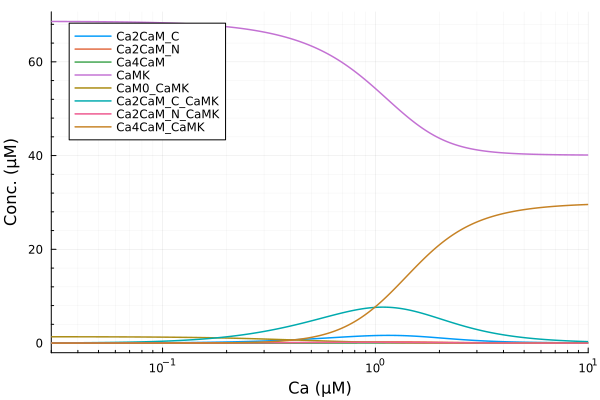
savefig("camkii_cam_binding.pdf")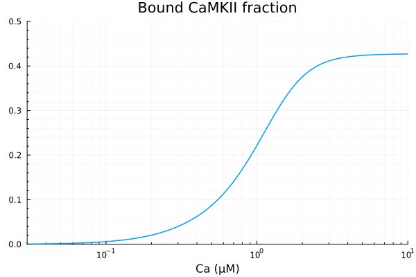
savefig("camkii_cam_binding.png")"/home/github/actions-runner-2/_work/camkii-cardiomyocyte-model/camkii-cardiomyocyte-model/docs/fits/camkii_cam_binding.png"We exclude CaMK bound with ApoCaM (CaM0_CaMK) from the active fraction.
CaMKAct = 1 - (sys.CaMK + sys.CaM0_CaMK) / sys.CAMKII_T
println("Basal activity with 30nM Ca is ", sim[1][CaMKAct])
xdata = ca
ydata = extract(sim, CaMKAct)
plot(xdata, ydata, label=false, title="Bound CaMKII fraction", ylims=(0, 0.5); xopts...)
Basal activity with 30nM Ca is 0.0005733354206699515
Old model fitting
Least-square fitting of steady state CaMKII activities against calcium concentrations.
Using a single Hill function to fit steady state CaMKII activities.
model_camk_single_hill(p, x) = @. p[1] * hil(x, p[2], p[4]) + p[3]
p0 = [0.4, 1μM, 0.0, 2.0]
prob = NonlinearCurveFitProblem(model_camk_single_hill, p0, xdata, ydata)
@time fit = solve(prob)

println("Basal activity: ", fit.u[3])
println("Maximal activated activity: ", fit.u[1])
println("Half-saturation Ca concentration: ", fit.u[2], " μM")
println("Hill coefficient: ", fit.u[4])
println("RMSE: ", mse(fit) |> sqrt)
3.630246 seconds (7.89 M allocations: 400.590 MiB, 2.18% gc time, 99.44% compilation time)
Basal activity: 0.005191064230946042
Maximal activated activity: 0.429964271164273
Half-saturation Ca concentration: 0.9630624525843235 μM
Hill coefficient: 2.298411998005468
RMSE: 0.004835726049863009
plot(xdata, [ydata predict(fit)], lab=["Full model" "Fitted"], line=[:dash :dot], title="Single Hill function fit", legend=:topleft, ylabel="Bound CaMKII fraction"; xopts...)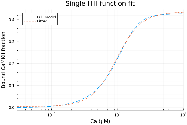
model_camk(p, x) = @. p[1] * hil(x, p[2], 2) + p[3] * hil(x, p[4], 4) + p[5]
p0 = [0.4, 1μM, 0.2, 1μM, 0.0]
prob = NonlinearCurveFitProblem(model_camk, p0, xdata, ydata)
@time fit = solve(prob)

println("Basal activity: ", fit.u[5])
println("Maximal activity by CaM-Ca2 binding: ", fit.u[1])
println("Half saturation Ca concentration for CaM-Ca2 binding: ", fit.u[2], " μM")
println("Maximal activity by CaM-Ca4 binding: ", fit.u[3])
println("Half saturation Ca concentration for CaM-Ca4 binding: ", fit.u[4], " μM")
println("RMSE: ", mse(fit) |> sqrt)
3.399406 seconds (8.38 M allocations: 423.670 MiB, 2.22% gc time, 99.77% compilation time)
Basal activity: 0.0010194269921517591
Maximal activity by CaM-Ca2 binding: 0.2651160783649847
Half saturation Ca concentration for CaM-Ca2 binding: 0.738524981625216 μM
Maximal activity by CaM-Ca4 binding: 0.16357325957465724
Half saturation Ca concentration for CaM-Ca4 binding: 1.2514899560431099 μM
RMSE: 0.0009704119533492081
plot(xdata, [ydata predict(fit)], lab=["Full model" "Fitted"], line=[:dash :dot], title="", legend=:topleft, ylabel="Bound CaMKII fraction"; xopts...)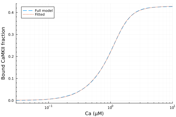
savefig("camkii_act_fit.pdf")
savefig("camkii_act_fit.png")"/home/github/actions-runner-2/_work/camkii-cardiomyocyte-model/camkii-cardiomyocyte-model/docs/fits/camkii_act_fit.png"Polynomial fitting
Using RationalPolynomialFitAlgorithm to fit the data with a rational polynomial function.
prob = CurveFitProblem(xdata, ydata)
alg = RationalPolynomialFitAlgorithm(num_degree=4, den_degree=4)
@time sol = solve(prob, alg)

println("Numerator coefficients: ", sol.u[1:5])
println("Denominator coefficients: ", vcat(1.0, sol.u[6:end]))
println("RMSE: ", mse(sol) |> sqrt)
2.655831 seconds (6.36 M allocations: 323.943 MiB, 98.94% compilation time)
Numerator coefficients: [0.00044199521336724286, -0.019900057595593965, 0.9342275027368985, -0.1638262371391244, 0.7550905642810347]
Denominator coefficients: [1.0, 2.9615924814344226, 1.270342014373002, -0.1934693320524475, 1.7554470156906479]
RMSE: 4.3975970066063445e-5
plot(xdata, [ydata sol.(xdata)], lab=["Full model" "Fitted"], line=[:dash :dot], title="Rational polynomial fit", legend=:topleft, ylabel="Bound CaMKII"; xopts...)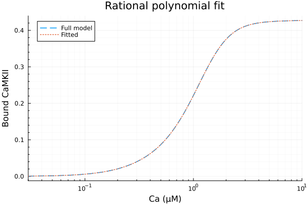
This notebook was generated using Literate.jl.