stochastic implementation (Gillespie SSA) of a collection of spontaneously decaying molecules.
using JumpProcesses
using Catalyst
using Plots

@time "Build system" rn738 = @reaction_network begin
    d, A --> 0
end

tend = 5.0
ps738 = Dict(:d => 1.0)
@time "Build problem" jprob1000 = JumpProblem(rn738, [:A => 1000], (0.0, tend), ps738)
jprob100 = remake(jprob1000, u0=[:A => 100])
jprob10 = remake(jprob1000, u0=[:A => 10])

@time "Solve problem" sol1000 = solve(jprob1000)
@time "Solve problem" sol100 = solve(jprob100)
@time "Solve problem" sol10 = solve(jprob10)
Build system: 0.013976 seconds (6.30 k allocations: 27.794 MiB, 68.20% compilation time)
Build problem: 8.872703 seconds (16.85 M allocations: 916.385 MiB, 5.77% gc time, 99.95% compilation time)
Solve problem: 0.266676 seconds (579.08 k allocations: 29.992 MiB, 99.96% compilation time)
Solve problem: 0.000037 seconds (232 allocations: 14.312 KiB)
Solve problem: 0.000028 seconds (48 allocations: 3.859 KiB)
retcode: Success
Interpolation: Piecewise constant interpolation
t: 12-element Vector{Float64}:
 0.0
 0.047428017939772825
 0.15633552354962163
 0.1579092594288904
 0.2207512309368772
 0.5678042572333265
 0.7037308503931872
 0.8519284866022026
 1.768681907789348
 2.4065061081127723
 2.614759226352355
 5.0
u: 12-element Vector{Vector{Int64}}:
 [10]
 [9]
 [8]
 [7]
 [6]
 [5]
 [4]
 [3]
 [2]
 [1]
 [0]
 [0]
plot(sol1000, xlabel="Time", ylabel="# of molecules", title="Fig. 7.38 (A)", label="1000 molecules")
plot!(t -> 1000 * exp(-t), linestyle=:dash, label="ODE solution")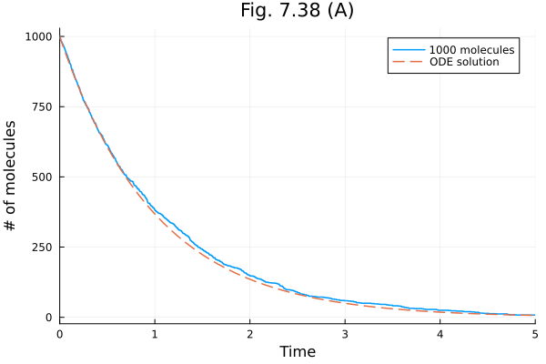
plot(sol100, xlabel="Time", ylabel="# of molecules", title="Fig. 7.38 (B)", label="100 molecules")
plot!(t -> 100 * exp(-t), linestyle=:dash, label="ODE solution")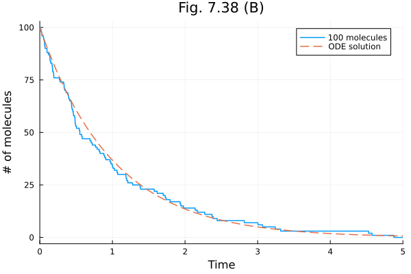
plot(sol10, xlabel="Time", ylabel="# of molecules", title="Fig. 7.38 (C)", label="10 molecules")
plot!(t -> 10 * exp(-t), linestyle=:dash, label="ODE solution")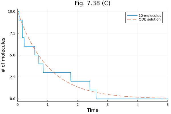
This notebook was generated using Literate.jl.