Chapter 1 - MMSB

Fig 1.7¶

Collins toggle switch model for Figures 1.7, 7.13, 7.14, 7.15.

using ModelingToolkit
using ModelingToolkit: t_nounits as t, D_nounits as D
using OrdinaryDiffEq
using Plots
Plots.gr(linewidth=1.5)

Plots.GRBackend()

function collins_sys(; name=:collins)
    @parameters a1=3 a2=2.5 β=4 γ=4
    @variables i1(t) i2(t) s1(t)=0.075 s2(t)=2.5
    hil(x, k) = x / (x + k)
    hil(x, k, n) = hil(x^n, k^n)
    eqs = [
        D(s1) ~ a1 * hil(1 + i2, s2, β) - s1,
        D(s2) ~ a2 * hil(1 + i1, s1, γ) - s2,
        i1 ~ 10 * (t > 30) * (t < 40),
        i2 ~ 10 * (t > 10) * (t < 20)
    ]
    return System(eqs, t; name)
end

collins_sys (generic function with 1 method)

tend = 50.0
@time "Build system" @mtkbuild sys = collins_sys()
@time "Build problem" prob = ODEProblem(sys, [], tend)
@time "Solve problem" sol = solve(prob, TRBDF2(), tstops=[10.0, 20.0, 30.0, 40.0])

Build system: 5.577399 seconds (11.33 M allocations: 557.772 MiB, 1.21% gc time, 99.86% compilation time: 91% of which was recompilation)
Build problem: 5.032466 seconds (24.57 M allocations: 1.223 GiB, 9.10% gc time, 99.66% compilation time: 55% of which was recompilation)
Solve problem: 0.068942 seconds (392.98 k allocations: 19.847 MiB, 97.38% compilation time)

retcode: Success
Interpolation: 3rd order Hermite
t: 56-element Vector{Float64}:
  0.0
  0.09225841921059712
  1.7526388801450203
  2.568311179460852
  8.493543764112186
 10.0
 10.0415187107798
 10.049822452935759
 10.132859874495356
 10.21657717872668
  ⋮
 35.3249197183359
 36.16490581885457
 36.793946822979365
 37.88905590907969
 38.73860510262759
 40.0
 41.450028364273194
 47.783398629187545
 50.0
u: 56-element Vector{Vector{Float64}}:
 [2.5, 0.075]
 [2.499993028589016, 0.07498972135990788]
 [2.499931328529461, 0.07490259985612023]
 [2.499925641113597, 0.07489622731058748]
 [2.4999205207461497, 0.07489135710870023]
 [2.4999212051748, 0.07489207387034473]
 [2.499902136359924, 0.1517377002582781]
 [2.499887884825495, 0.17522507057840955]
 [2.4977211764961, 0.3997377735356334]
 [2.4840179326347935, 0.6079865813051137]
 ⋮
 [2.4885009769559527, 0.10717550906807255]
 [2.4951713353678695, 0.08897384338141681]
 [2.497454073733895, 0.08251061304997978]
 [2.499201951475437, 0.07739503387098845]
 [2.499668465434689, 0.07596341029268566]
 [2.499893894545783, 0.0751748928762065]
 [2.4999163130304596, 0.07494006253473165]
 [2.4999223238789505, 0.07488300375283861]
 [2.499921397869864, 0.07489186510360883]

plot(sol, title="Fig. 1.7", xlabel="Time", ylabel="Concentration")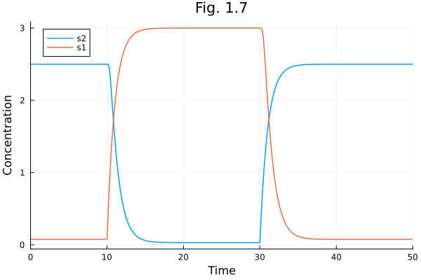

plot(sol, idxs=[sys.i1, sys.i2], labels=["i1" "i2"], xlabel="Time", ylabel="Signal strength")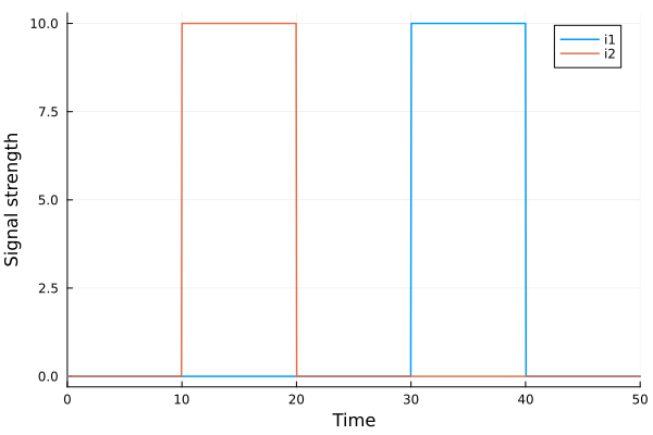

Fig 1.09¶

Hodgkin-Huxley model

using OrdinaryDiffEq
using ModelingToolkit
using ModelingToolkit: t_nounits as t, D_nounits as D
using Plots
Plots.gr(linewidth=1.5)

Plots.GRBackend()

function hh_sys(; name=:hh)
    exprel(x) = x / expm1(x)
    @discretes iStim(t)=0.0
    @parameters E_N=55 E_K=-72 E_LEAK=-49 G_N_BAR=120 G_K_BAR=36 G_LEAK=0.3 C_M=1
    @variables v(t)=-59.8977 m(t)=0.0536 h(t)=0.5925 n(t)=0.3192 iNa(t) iK(t) iLeak(t) ma(t) mb(t) ha(t) hb(t) na(t) nb(t)

    # Electrical stimulation events
    stim_on_1 = ModelingToolkit.SymbolicDiscreteCallback([20.0] => [iStim ~ -6.6], discrete_parameters = iStim, iv = t)
    stim_off_1 = ModelingToolkit.SymbolicDiscreteCallback([21.0] => [iStim ~ 0.0], discrete_parameters = iStim, iv = t)
    stim_on_2 = ModelingToolkit.SymbolicDiscreteCallback([60.0] => [iStim ~ -6.9], discrete_parameters = iStim, iv = t)
    stim_off_2 = ModelingToolkit.SymbolicDiscreteCallback([61.0] => [iStim ~ 0.0], discrete_parameters = iStim, iv = t)

    eqs = [
        ma ~ exprel(-0.10 * (v + 35)),
        mb ~ 4.0 * exp(-(v + 60) / 18.0),
        ha ~ 0.07 * exp(-(v + 60) / 20),
        hb ~ 1 / (exp(-(v + 30) / 10) + 1),
        na ~ 0.1 * exprel(-0.1 * (v + 50)),
        nb ~ 0.125 * exp(-(v + 60) / 80),
        iNa ~ G_N_BAR * (v - E_N) * (m^3) * h,
        iK ~ G_K_BAR * (v - E_K) * (n^4),
        iLeak ~ G_LEAK * (v - E_LEAK),
        D(v) ~ -(iNa + iK + iLeak + iStim) / C_M,
        D(m) ~ -(ma + mb) * m + ma,
        D(h) ~ -(ha + hb) * h + ha,
        D(n) ~ -(na + nb) * n + na
    ]
    sys = ODESystem(eqs, t; name, discrete_events=[stim_on_1, stim_off_1, stim_on_2, stim_off_2])
    return sys
end

hh_sys (generic function with 1 method)

tend = 100.0
@time "Build system" @mtkcompile sys = hh_sys()
@time "Build problem" prob = ODEProblem(sys, [], tend)
@time "Solve problem" sol = solve(prob, TRBDF2())

Build system: 1.693994 seconds (7.42 M allocations: 369.855 MiB, 2.33% gc time, 98.98% compilation time: 1% of which was recompilation)
Build problem: 2.817898 seconds (6.10 M allocations: 312.765 MiB, 1.61% gc time, 99.01% compilation time)
Solve problem: 5.257778 seconds (19.17 M allocations: 1000.897 MiB, 1.69% gc time, 99.84% compilation time: <1% of which was recompilation)

retcode: Success
Interpolation: 3rd order Hermite
t: 86-element Vector{Float64}:
   0.0
   0.043933380198988056
   0.8603019183785529
   1.4238266341729466
   4.248524319244266
   7.256696580279218
  14.008668650102734
  20.0
  20.0
  20.523672537957506
   ⋮
  80.98994690756788
  82.75533576957824
  85.28523794002348
  87.0567951172999
  89.58671291457803
  92.11663071185616
  95.36073853933443
  98.60484636681271
 100.0
u: 86-element Vector{Vector{Float64}}:
 [0.3192, 0.5925, 0.0536, -59.8977]
 [0.31920037837610854, 0.5925001823589415, 0.05359578382735057, -59.89751905826826]
 [0.3192092568010022, 0.5924998590652717, 0.05358184355412253, -59.89566008856614]
 [0.3192163677409184, 0.5924970879076324, 0.05358943258416223, -59.8950814157433]
 [0.3192459341881293, 0.5924809146952184, 0.053592196231923135, -59.89502830986493]
 [0.31925609549509726, 0.5924817912524404, 0.05357830777581423, -59.8972639308857]
 [0.31924376588366404, 0.5925213611499963, 0.05356958137228632, -59.89841215473991]
 [0.3192437144541843, 0.5925326003276699, 0.05357583828365716, -59.897458016671024]
 [0.3192437144541843, 0.5925326003276699, 0.05357583828365716, -59.897458016671024]
 [0.32155917317121, 0.5890432009452047, 0.06551860167610044, -56.81727065722307]
 ⋮
 [0.31139247790487395, 0.6031106305241054, 0.052022691780803584, -60.03624850802009]
 [0.3142669515137392, 0.6000691383062857, 0.05586512301488734, -59.48738732983398]
 [0.3190176931317737, 0.5935667912021315, 0.057101906306891784, -59.36939888583165]
 [0.32089630293403637, 0.590555970243717, 0.055813136707009416, -59.58538988535853]
 [0.32106895880988423, 0.5898014922646461, 0.05365651750240197, -59.909782135516984]
 [0.3199015194882542, 0.5912671247973527, 0.052748041474315874, -60.032332929045424]
 [0.318868838187065, 0.592858729636698, 0.053072218741163794, -59.96919401789336]
 [0.3188802294577743, 0.5930203127977014, 0.053645771949752334, -59.88204595309853]
 [0.31904457349408305, 0.592822868458166, 0.053752588605212086, -59.86802351279653]

plot(sol, idxs=[sys.v], xlabel="Time (ms)", ylabel="Membrane potential (mV)", title="Fig 1.9")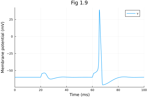

This notebook was generated using Literate.jl.