Chapter 2 - MMSB

Fig 2.04¶

Exponential decay

using Startup

using Plots
Plots.default(linewidth=1.5)

pl = plot(xlabel="Time", ylabel="Concentration", title="Fig 2.4")
for k in 1:3
    plot!(pl, t -> 3 * exp(-k * t), 0, 5, label="exp(-$(k)t)")
end
pl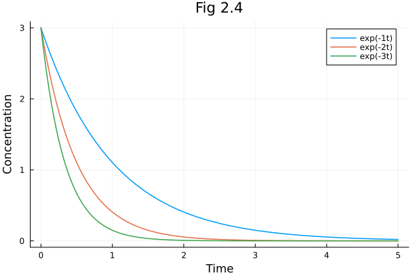

Fig 2.09¶

Metabolic network simulation

using OrdinaryDiffEq
using Catalyst
using Plots

@time "Build system" rn209 = @reaction_network model209 begin
    k1, 0 --> A
    k2, A --> B
    k3, A + B --> C + D
    k4, C --> 0
    k5, D --> 0
end

Build system: 5.288586 seconds (7.98 M allocations: 561.075 MiB, 3.60% gc time, 99.93% compilation time: 97% of which was recompilation)

up209 = (:k1 => 3.0, :k2 => 2.0, :k3 => 2.5, :k4 => 3.0, :k5 => 4.0, :A => 0.0, :B => 0.0, :C => 0.0, :D => 0.0)
tend = 10.0
@time "Build problem" prob209 = ODEProblem(rn209, up209, tend)
@time "Solve problem" sol = solve(prob209, Tsit5())
plot(sol, title="Fig 2.9", xlabel="Time", ylabel="Concentration")

Build problem: 36.556973 seconds (39.40 M allocations: 2.739 GiB, 3.69% gc time, 99.84% compilation time: 32% of which was recompilation)
Solve problem: 2.251438 seconds (4.37 M allocations: 306.400 MiB, 2.67% gc time, 99.83% compilation time)

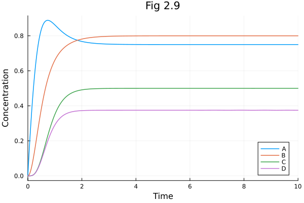
Figure 2.11¶

Intro to model reduction of ODE metabolic networks.

using OrdinaryDiffEq
using Catalyst
using Plots

@time "Build system" rn211 = @reaction_network model211 begin
    k0, 0 --> A
    (k1, km1), A <--> B
    k2, B --> 0
end

Build system: 0.000634 seconds (1.24 k allocations: 60.914 KiB)

up211 = (:k0 => 0.0, :k1 => 9.0, :km1 => 12.0, :k2 => 2.0, :A => 0.0, :B => 10.0)
tend = 3.0
@time "Build problem" prob211 = ODEProblem(rn211, up211, tend)
@time "Solve problem" sol211 = solve(prob211, Tsit5())
plot(sol211, title="Fig 2.11", xlabel="Time", ylabel="Concentration")

Build problem: 1.233556 seconds (2.06 M allocations: 146.358 MiB, 3.45% gc time, 97.80% compilation time)
Solve problem: 0.661124 seconds (920.35 k allocations: 64.943 MiB, 6.53% gc time, 99.52% compilation time)

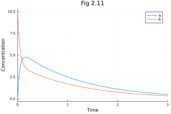
Figure 2.12¶

Rapid equilibrium assumption

@time "Build system" rn212 = @reaction_network model212 begin
    @parameters k0 k1 km1 k2
    @equations begin
        A ~ C * km1 / (km1 + k1)
        B ~ C * k1 / (km1 + k1)
    end
    k0, 0 --> C
    k2 * k1 / (km1 + k1), C --> 0
end

Build system: 0.488571 seconds (249.11 k allocations: 17.121 MiB, 99.56% compilation time: 3% of which was recompilation)

tend = 3.0
up212 = (:k0 => 0.0, :k1 => 9.0, :km1 => 12.0, :k2 => 2.0, :C => 10.0)
@time "Build problem" prob212 = ODEProblem(rn212, up212, tend; mtkcompile=true)
@time "Solve problem" sol212 = solve(prob212, Tsit5())

plot(sol211, linestyle=:dash, label=["A (Full model)" "B (Full model)"])
plot!(sol212, idxs=[:A, :B], linestyle=:solid, label=["A (Reduced model)" "B (Reduced model)"])
plot!(title="Fig 2.12", xlabel="Time", ylabel="Concentration")

Build problem: 2.413230 seconds (2.97 M allocations: 215.588 MiB, 1.72% gc time, 98.61% compilation time: 22% of which was recompilation)
Solve problem: 0.625377 seconds (902.02 k allocations: 63.892 MiB, 6.12% gc time, 99.50% compilation time)

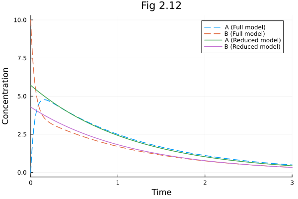
Figure 2.13¶

When another set of parameters breaks rapid equilibrium assumption.

pmap213 = Dict(:k0=>9.0, :k1=>21.0, :km1=>12.0, :k2=>2.0)
u0map213 = Dict(:A=>8.0, :B=>4.0)
tend = 3.0
prob213full = remake(prob211; p=pmap213, u0=u0map213, tspan=(0.0, tend))
prob213re = ODEProblem(rn212, (:C=>12.0), tend, pmap213; mtkcompile=true)
@time sol213full = solve(prob213full, Tsit5())
@time sol213re = solve(prob213re, Tsit5())

plot(sol213full,  linestyle=:dash, label=["A (Full model)" "B (Full model)"])
plot!(sol213re, idxs=[:A, :B], linestyle=:solid, label=["A (Reduced model)" "B (Reduced model)"])
plot!(title="Fig 2.13", xlabel="Time", ylabel="Concentration")

  0.000396 seconds (621 allocations: 47.414 KiB)
  0.000413 seconds (371 allocations: 25.586 KiB)

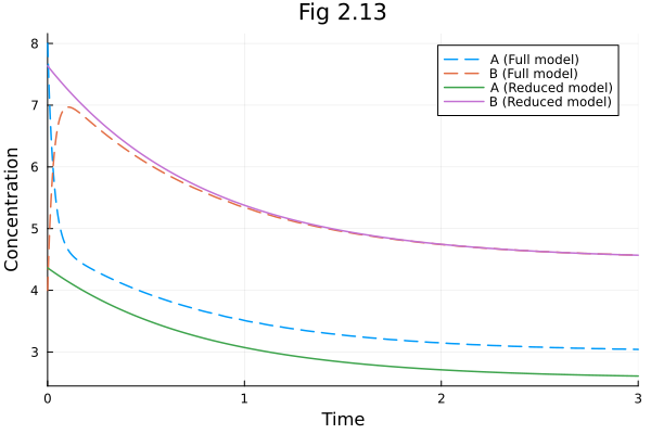
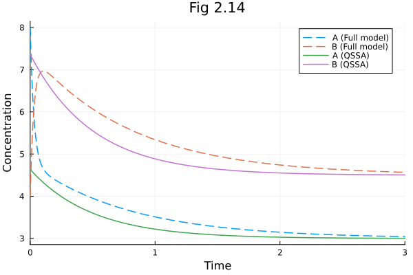
Figure 2.14¶

Quasi-steady state assumption on species A (D(A) ~ 0). You can model this in Catalyst.jl DSL like:

@time "Build system" rn214 = @reaction_network model214 begin
    @parameters k0=9 k1=21 km1=12 k2=2
    @variables A(t)
    @equations begin
        A ~ (k0 + km1 * B) / k1
    end
    (k1 * A, (k2 + km1)), 0 <--> B
end

Build system: 0.053121 seconds (23.67 k allocations: 1.570 MiB, 96.53% compilation time)

Or use ModelingToolkit.jl equations to set dA ~ 0 directly. The QSS concentrations of A

using ModelingToolkit

function model214(u0; name=:model214)
    @independent_variables t
    @parameters k0=9 k1=21 km1=12 k2=2

    D = Differential(t)
    @variables A(t) B(t) = (k1 * u0 - k0) / (km1 + k1)

    v0 = k0
    v1 = k1 * A - km1 * B
    v2 = k2 * B
    dA = v0 - v1
    dB = v1 - v2

    eqs = [
        0 ~ dA, ## Quasi-steady state assumption on species A (`D(A) ~ 0`)
        D(B) ~ dB,
    ]
    return ODESystem(eqs, t; name)
end

tend = 3.0
@time "Build system" @mtkcompile sys214 = model214(12.0)
@time "Build problem" prob214 = ODEProblem(sys214, [], (0.0, tend))

Build system: 0.283489 seconds (23.61 k allocations: 1.279 MiB, 96.76% compilation time)
Build problem: 1.187940 seconds (1.20 M allocations: 88.815 MiB, 4.67% gc time, 97.27% compilation time: 38% of which was recompilation)

ODEProblem with uType Vector{Float64} and tType Float64. In-place: true
Initialization status: FULLY_DETERMINED
Non-trivial mass matrix: false
timespan: (0.0, 3.0)
u0: 1-element Vector{Float64}:
 7.363636363636363

equations(sys214)

observed(sys214)

@time "Solve problem" sol214 = solve(prob214, Tsit5())
@unpack A, B = sys214

plot(sol213full, linestyle=:dash, label=["A (Full model)" "B (Full model)"])
plot!(sol214, idxs=[A, B], linestyle=:solid, label=["A (QSSA)" "B (QSSA)"])
plot!(title="Fig 2.14", xlabel="Time", ylabel="Concentration")

Solve problem: 0.643860 seconds (824.57 k allocations: 58.456 MiB, 99.35% compilation time)

Problem 2.4.6¶

using OrdinaryDiffEq
using Plots

sol246 = ODEProblem((u, p, t) -> p * (1.0 - u), 0.0, 10.0, 1.0) |> solve
plot(sol246, title="Problem 2.4.6", xlabel="Time", ylabel="Concentration")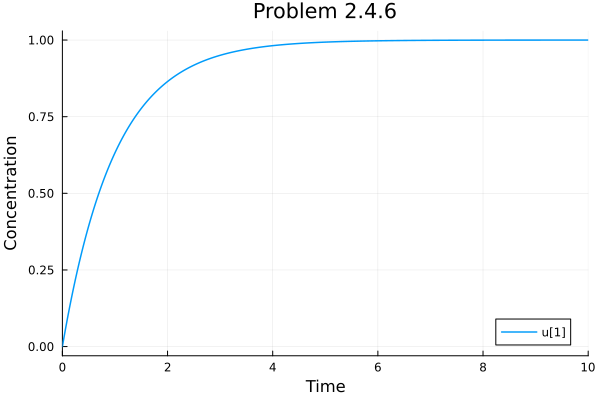

This notebook was generated using Literate.jl.