Chapter 4 - MMSB

using Startup

using OrdinaryDiffEq
using Catalyst
using ModelingToolkit
using ModelingToolkit: t_nounits as t, D_nounits as D
using Plots
Plots.gr(linewidth=1.5)

Plots.GRBackend()

Convenience functions to plot gradients of the ODEs.

function meshgrid(xrange, yrange)
    xx = [x for y in yrange, x in xrange]
    yy = [y for y in yrange, x in xrange]
    return xx, yy
end

"Get the gradients of the vector field of an ODE system at a grid of points in the state space."
function get_gradient(prob, xsym, ysym, xx, yy; t = nothing)
    # The order of state variables (unknowns) in the ODE system is not guaranteed. So we may need to swap the order of x and y when calling ∂F.
    swap_or_not(x, y; xidx=1) = xidx == 1 ? [x, y] : [y, x]
    ∂F = prob.f
    ps = prob.p
    sys = prob.f.sys
    xidx = ModelingToolkit.variable_index(sys, xsym)
    yidx = ModelingToolkit.variable_index(sys, ysym)
    dx = map((x, y) -> ∂F(swap_or_not(x, y; xidx), ps, t)[xidx], xx, yy)
    dy = map((x, y) -> ∂F(swap_or_not(x, y; xidx), ps, t)[yidx], xx, yy)
    return (dx, dy)
end

function normalize_gradient(dx, dy, xscale, yscale; transform=cbrt)
    maxdx = maximum(abs, dx)
    maxdy = maximum(abs, dy)
    dx_norm = @. transform(dx / maxdx) * xscale
    dy_norm = @. transform(dy / maxdy) * yscale
    return (dx_norm, dy_norm)
end

normalize_gradient (generic function with 1 method)

Fig 4.2 A¶

@time "Build system" rn402 = @reaction_network begin
    k1 / (1 + B^n), 0 --> A
    k2, 0 --> B
    k3, A --> 0
    k4, B --> 0
    k5, A --> B
end

Build system: 0.147287 seconds (319.78 k allocations: 26.995 MiB, 98.60% compilation time)

up402 = Dict(:k1 => 20.0, :k2 => 5.0, :k3 => 5.0, :k4 => 5.0, :k5 => 2.0, :n => 4.0, :A => 0.0, :B => 0.0)
tend = 1.5
@time "Build problem" prob402 = ODEProblem(rn402, up402, tend)
u0s = [
    [0.0, 0.0],
    [0.5, 0.6],
    [0.17, 1.1],
    [0.25, 1.9],
    [1.85, 1.7]
]

Build problem: 0.835219 seconds (1.75 M allocations: 126.985 MiB, 2.75% gc time, 96.70% compilation time)

5-element Vector{Vector{Float64}}:
 [0.0, 0.0]
 [0.5, 0.6]
 [0.17, 1.1]
 [0.25, 1.9]
 [1.85, 1.7]

@time sols = map(u0s) do u0
    solve(remake(prob402, u0=u0), TRBDF2())
end
plot(sols[1], xlabel="Time", ylabel="Concentration", title="Fig. 4.2 A")

  0.813043 seconds (1.15 M allocations: 81.065 MiB, 4.15% gc time, 99.41% compilation time)

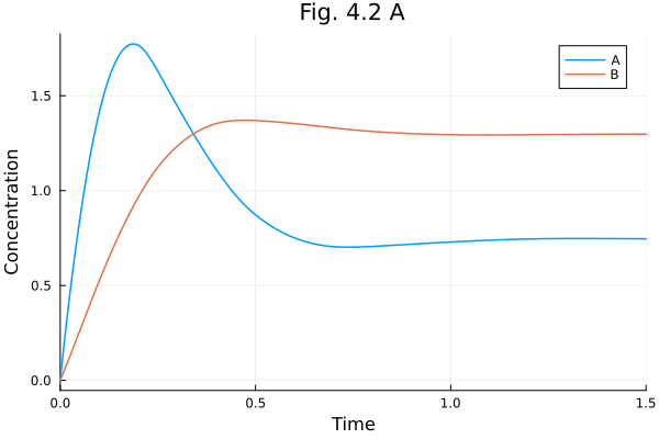
Fig. 4.2 B (Phase plot)¶

@unpack A, B = rn402
plot(sols[1], idxs=(A, B), xlabel="Time", ylabel="Concentration", title="Fig. 4.2 B", aspect_ratio=1, size=(600, 600), label=false, xlims=(0, 2), ylims=(0, 2))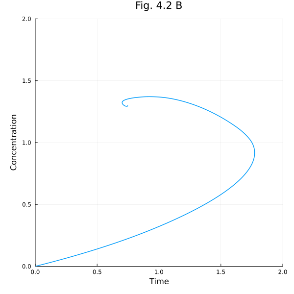

Fig. 4.3 A (Multiple time series)¶

plot(xlabel="Time", ylabel="Concentration")
for sol in sols
    plot!(sol, label=false)
end
plot!(title="Fig. 4.3 A")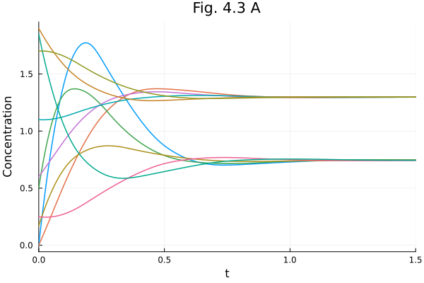

Fig. 4.3 B (Phase plot)¶

plot(xlabel="[A]", ylabel="[B]")
for sol in sols
    plot!(sol, idxs=(A, B), label=false)
end
plot!(title="Fig. 4.3 B", aspect_ratio=1, size=(600, 600), xlims=(0, 2), ylims=(0, 2))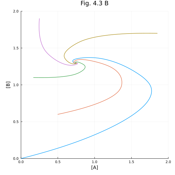

Fig. 4.4 A¶

Let’s sketch vector fields in phase plots.

xrange = 0:0.1:2
yrange = 0:0.1:2

xx, yy = meshgrid(xrange, yrange)
dx, dy = get_gradient(prob402, A, B, xx, yy)
dx_norm, dy_norm = normalize_gradient(dx, dy, step(xrange), step(yrange))
quiver(xx, yy, quiver=(dx_norm, dy_norm), color=:gray)

for sol in sols
    plot!(sol, idxs=(A, B), label=false)
end

plot!(title="Fig. 4.4 A", aspect_ratio=1, size=(600, 600), xlims=(0, 2), ylims=(0, 2))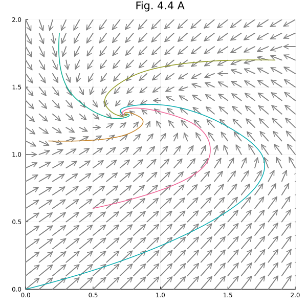

Figure 4.5A¶

Nullclines

xrange = 0:0.01:2
yrange = 0:0.01:2
xx, yy = meshgrid(xrange, yrange)
dx, dy = get_gradient(prob402, A, B, xx, yy)

contour(xrange, yrange, dx, levels=[0], line=(:black, :solid), colorbar=false)
plot!([], [],  line=(:black, :solid), label="A nullcline")
contour!(xrange, yrange, dy, levels=[0], line=(:black, :dash), colorbar=false)
plot!([], [], line=(:black, :dash), label="B nullcline")
for sol in sols
    plot!(sol, idxs=(A, B), label=false)
end

plot!(title="Fig. 4.5 A", aspect_ratio=1, size=(600, 600), xlims=(0, 2), ylims=(0, 2), xlabel="[A]", ylabel="[B]", legend=:bottomright)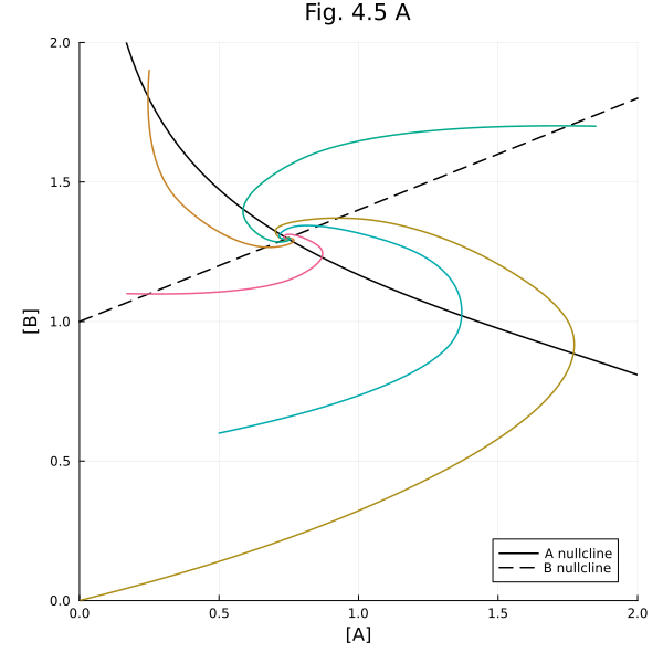

Figure 4.5 B¶

Vector field with nullclines.

xrange = 0:0.01:2
yrange = 0:0.01:2
xx, yy = meshgrid(xrange, yrange)
dx, dy = get_gradient(prob402, A, B, xx, yy)

xx_sp = xx[1:10:end, 1:10:end]
yy_sp = yy[1:10:end, 1:10:end]
dx_sp = dx[1:10:end, 1:10:end]
dy_sp = dy[1:10:end, 1:10:end]
dx_sp_norm, dy_sp_norm = normalize_gradient(dx_sp, dy_sp, step(xrange)*10, step(yrange)*10)
quiver(xx_sp, yy_sp, quiver=(dx_sp_norm, dy_sp_norm), color=:gray)
contour!(xrange, yrange, dx, levels=[0], line=(:black, :solid), colorbar=false)
plot!([], [],  line=(:black, :solid), label="A nullcline")
contour!(xrange, yrange, dy, levels=[0], line=(:black, :dash), colorbar=false)
plot!([], [], line=(:black, :dash), label="B nullcline")
plot!(title="Fig. 4.5 B", aspect_ratio=1, size=(600, 600), xlims=(0, 2), ylims=(0, 2), xlabel="[A]", ylabel="[B]", legend=:bottomright)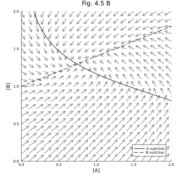

Fig 4.7 A¶

Symmetric (bistable) biological networks.

@time "Build system" rn407 = @reaction_network begin
    k1 / (1 + B^n1), 0 --> A
    k2 / (1 + A^n2), 0 --> B
    k3, A --> 0
    k4, B --> 0
end

Build system: 0.000836 seconds (1.52 k allocations: 70.539 KiB)

up407 = Dict(:k1 => 20.0, :k2 => 20.0, :k3 => 5.0, :k4 => 5.0, :n1 => 4.0, :n2 => 1.0, :A => 3.0, :B => 1.0)
tend = 4.0
@time "Build problem" prob407 = ODEProblem(rn407, up407, (0.0, tend))
@time sol1 = solve(prob407, TRBDF2())
@time sol2 = solve(remake(prob407, u0=[:A => 1.0, :B => 3.0]), TRBDF2())
pl1 = plot(sol1, xlabel="Time", ylabel="Concentration", title="Fig 4.7A (1)")
pl2 = plot(sol2, xlabel="Time", ylabel="Concentration", title="Fig 4.7A (2)")
plot(pl1, pl2, layout=(2, 1))

Build problem: 0.309685 seconds (690.23 k allocations: 49.979 MiB, 95.17% compilation time)
  0.462790 seconds (493.78 k allocations: 35.227 MiB, 5.40% gc time, 99.79% compilation time)
  3.608474 seconds (3.69 M allocations: 263.019 MiB, 1.61% gc time, 99.46% compilation time)

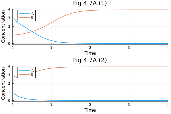
Fig 4.7 B¶

Vector field with nullclines

xrange = range(0, 5, 201)
yrange = range(0, 5, 201)
xx, yy = meshgrid(xrange, yrange)
dx, dy = get_gradient(prob407, A, B, xx, yy)
xx_sp = xx[1:10:end, 1:10:end]
yy_sp = yy[1:10:end, 1:10:end]
dx_sp = dx[1:10:end, 1:10:end]
dy_sp = dy[1:10:end, 1:10:end]
dx_sp_norm, dy_sp_norm = normalize_gradient(dx_sp, dy_sp, step(xrange)*10, step(yrange)*10)
quiver(xx_sp, yy_sp, quiver=(dx_sp_norm, dy_sp_norm), color=:gray)
contour!(xrange, yrange, dx, levels=[0], line=(:black, :solid), colorbar=false)
plot!([], [],  line=(:black, :solid), label="A nullcline")
contour!(xrange, yrange, dy, levels=[0], line=(:black, :dash), colorbar=false)
plot!([], [], line=(:black, :dash), label="B nullcline")
plot!(title="Fig. 4.7B", aspect_ratio=1, size=(600, 600), xlims=(0, 5), ylims=(0, 5), xlabel="[A]", ylabel="[B]", legend=:topright)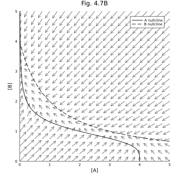

Fig 4.8 A¶

Symmetric parameter set

prob408 = remake(prob407, p=[:k1 => 20.0, :k2 => 20.0, :k3 => 5.0, :k4 => 5.0, :n1 => 4.0, :n2 => 4.0], u0=[:A => 3.0, :B => 1.0], tspan=(0.0, 4.0))
@time sol1 = solve(prob408, TRBDF2())
@time sol2 = solve(remake(prob408, u0=[:A => 1.0, :B => 3.0]), TRBDF2())
pl1 = plot(sol1, xlabel="Time", ylabel="Concentration", title="Fig 4.8A (1)")
pl2 = plot(sol2, xlabel="Time", ylabel="Concentration", title="Fig 4.8A (2)")
plot(pl1, pl2, layout=(2, 1))

  0.000509 seconds (402 allocations: 29.781 KiB)
  0.007085 seconds (21.06 k allocations: 1.271 MiB)

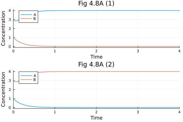
Fig 4.8 B¶

Nullclines and vector field

@unpack A, B = prob408.f.sys

xrange = range(0, 5, 201)
yrange = range(0, 5, 201)
xx, yy = meshgrid(xrange, yrange)
dx, dy = get_gradient(prob408, A, B, xx, yy)
xx_sp = xx[1:10:end, 1:10:end]
yy_sp = yy[1:10:end, 1:10:end]
dx_sp = dx[1:10:end, 1:10:end]
dy_sp = dy[1:10:end, 1:10:end]
dx_sp_norm, dy_sp_norm = normalize_gradient(dx_sp, dy_sp, step(xrange)*10, step(yrange)*10)
quiver(xx_sp, yy_sp, quiver=(dx_sp_norm, dy_sp_norm), color=:gray)
contour!(xrange, yrange, dx, levels=[0], line=(:black, :solid), colorbar=false)
plot!([], [],  line=(:black, :solid), label="A nullcline")
contour!(xrange, yrange, dy, levels=[0], line=(:black, :dash), colorbar=false)
plot!([], [], line=(:black, :dash), label="B nullcline")
plot!(title="Fig. 4.8 B", aspect_ratio=1, size=(600, 600), xlims=(0, 5), ylims=(0, 5), xlabel="[A]", ylabel="[B]", legend=:topright)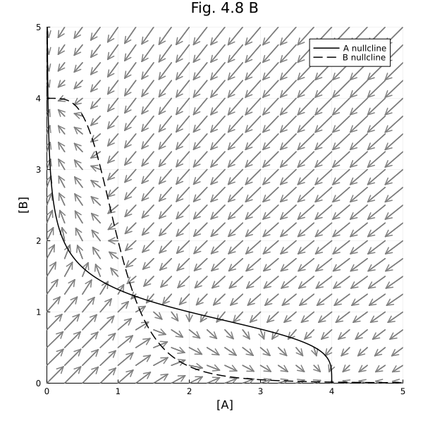

Fig 4.8 C¶

Around the unstable steady-state.

xrange = 1.0:0.01:1.5
yrange = 1.0:0.01:1.5
xx, yy = meshgrid(xrange, yrange)
dx, dy = get_gradient(prob408, A, B, xx, yy)
xx_sp = xx[1:5:end, 1:5:end]
yy_sp = yy[1:5:end, 1:5:end]
dx_sp = dx[1:5:end, 1:5:end]
dy_sp = dy[1:5:end, 1:5:end]
dx_sp_norm, dy_sp_norm = normalize_gradient(dx_sp, dy_sp, step(xrange)*5, step(yrange)*5)
quiver(xx_sp, yy_sp, quiver=(dx_sp_norm, dy_sp_norm), color=:gray)
contour!(xrange, yrange, dx, levels=[0], line=(:black, :solid), colorbar=false)
plot!([], [],  line=(:black, :solid), label="A nullcline")
contour!(xrange, yrange, dy, levels=[0], line=(:black, :dash), colorbar=false)
plot!([], [], line=(:black, :dash), label="B nullcline")
plot!(title="Fig. 4.8 C", aspect_ratio=1, size=(600, 600), xlims=(1.0, 1.5), ylims=(1.0, 1.5), xlabel="[A]", ylabel="[B]", legend=:topright)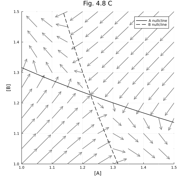

Another way to draw nullclines is to find the analytical solutions for dA (or dB) is zero. And then sketch the nullclines in a parameteric plot.

nca47(b, p) = p.k1 / p.k3 / (1 + b^p.n1)
ncb47(a, p) = p.k2 / p.k4 / (1 + a^p.n2)

pls = map((8.0, 16.0, 20.0, 35.0)) do k1
    ps = (k1=k1, k2=20., k3=5., k4=5., n1=4., n2=4.)
    pl = plot(t->nca47(t, ps), identity, 0, 7, color=:red, label="Nullcline A")
    plot!(pl, identity, t->ncb47(t, ps), 0, 7, color=:blue, label="Nullcline B")
    plot!(xlims=(0, 7), ylims=(0, 7), aspect_ratio=1, title="k1 = $k1", xlabel="[A]", ylabel="[B]", legend=:right)
end

plot(pls..., layout=(2, 2), size=(800, 800))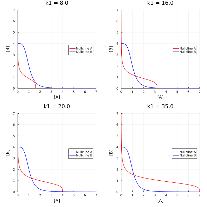

Fig 4.11¶

Surface plots

using Plots
z1(x, y) = x^2 + 0.5y^2
z2(x, y) = (.2x^2-1)^2 + y^2
x1 = y1 = range(-1.0, 1.0, 41)
x2 = range(-2.75, 2.75, 41)
y2 = range(-0.75, 0.75, 41)
p1 = surface(x1, y1, z1, title="Single-well potential")
p2 = contourf(x1, y1, z1)
p3 = surface(x2, y2, z2, title="Double-well potential")
p4 = contourf(x2, y2, z2)
plot(p1, p2, p3, p4, size=(800, 600))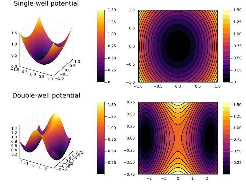

Fig 4.15 A¶

Oscillatory networks

using Catalyst
using OrdinaryDiffEq
using Plots
Plots.gr(linewidth=1.5)

Plots.GRBackend()

@time "Build system" model415 = @reaction_network begin
    k0 , 0 --> A
    k1 * (1 + B^n), A --> B
    k2, B --> 0
end

Build system: 0.000801 seconds (1.18 k allocations: 57.789 KiB)

up415 = Dict(:k0 => 8.0, :k1 => 1.0, :k2 => 5.0, :n => 2.0, :A => 1.5, :B => 1.0)
tend = 8.0
@time "Build problem" prob415 = ODEProblem(model415, up415, (0.0, tend))

u0s = [
    [:A=>1.5, :B=>1.0],
    [:A=>0.0, :B=>1.0],
    [:A=>0.0, :B=>3.0],
    [:A=>2.0, :B=>0.0],
]

@time "Solve problems" sols = map(u0s) do u0
    solve(remake(prob415, u0=u0), TRBDF2())
end

plot(sols[1], xlabel="Time", ylabel="Concentration", title="Fig. 4.15 A")

Build problem: 0.646061 seconds (1.05 M allocations: 77.744 MiB, 95.24% compilation time)
Solve problems: 1.146061 seconds (1.31 M allocations: 91.305 MiB, 2.75% gc time, 97.66% compilation time)

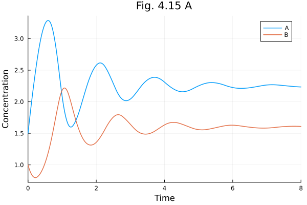
Fig 4.15 B¶

Vector field with nullclines

xrange = range(0, 4, 101)
yrange = range(0, 4, 101)
xx, yy = meshgrid(xrange, yrange)
dx, dy = get_gradient(prob415, :A, :B, xx, yy)
xx_sp = xx[1:5:end, 1:5:end]
yy_sp = yy[1:5:end, 1:5:end]
dx_sp = dx[1:5:end, 1:5:end]
dy_sp = dy[1:5:end, 1:5:end]
dx_sp_norm, dy_sp_norm = normalize_gradient(dx_sp, dy_sp, step(xrange)*5, step(yrange)*5)
quiver(xx_sp, yy_sp, quiver=(dx_sp_norm, dy_sp_norm), color=:gray)

for sol in sols
    plot!(sol, idxs=(:A, :B), label=false)
end

contour!(xrange, yrange, dx, levels=[0], line=(:black, :solid), colorbar=false)
plot!([], [],  line=(:black, :solid), label="A nullcline")
contour!(xrange, yrange, dy, levels=[0], line=(:black, :dash), colorbar=false)
plot!([], [], line=(:black, :dash), label="B nullcline", legend=:bottomright)
plot!(title="Fig. 4.15 B", aspect_ratio=1, size=(600, 600), xlims=(0, 4), ylims=(0, 4), xlabel="[A]", ylabel="[B]", legend=:bottomright)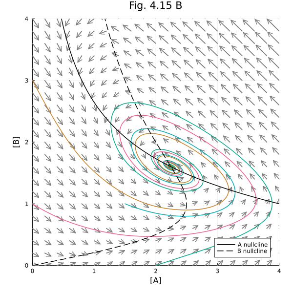

Fig 4.16 A¶

Oscillatory parameter set

prob416 = remake(prob415, p=[:n=>2.5], tspan=(0.0, 100.0))
@time "Solve problems" sols = map(u0s) do u0
    solve(remake(prob416, u0=u0), TRBDF2())
end

plot(sols[1], xlabel="Time", ylabel="Concentration", title="Fig. 4.16 A", tspan=(0.0, 10.0))

Solve problems: 0.093637 seconds (114.51 k allocations: 7.194 MiB, 64.90% compilation time)

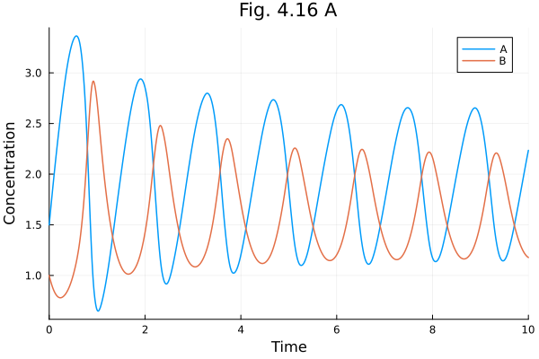
Fig 4.16 B¶

xrange = range(0, 4, 201)
yrange = range(0, 4, 201)
xx, yy = meshgrid(xrange, yrange)
dx, dy = get_gradient(prob416, :A, :B, xx, yy)
xx_sp = xx[1:10:end, 1:10:end]
yy_sp = yy[1:10:end, 1:10:end]
dx_sp = dx[1:10:end, 1:10:end]
dy_sp = dy[1:10:end, 1:10:end]
dx_sp_norm, dy_sp_norm = normalize_gradient(dx_sp, dy_sp, step(xrange)*10, step(yrange)*10)
quiver(xx_sp, yy_sp, quiver=(dx_sp_norm, dy_sp_norm), color=:gray)

for sol in sols
    plot!(sol, idxs=(:A, :B), label=false)
end

contour!(xrange, yrange, dx, levels=[0], line=(:black, :solid), colorbar=false)
plot!([], [],  line=(:black, :solid), label="A nullcline")
contour!(xrange, yrange, dy, levels=[0], line=(:black, :dash), colorbar=false)
plot!([], [], line=(:black, :dash), label="B nullcline", legend=:bottomright)
plot!(title="Fig. 4.16 B", aspect_ratio=1, size=(600, 600), xlims=(0, 4), ylims=(0, 4), xlabel="[A]", ylabel="[B]", legend=:topright)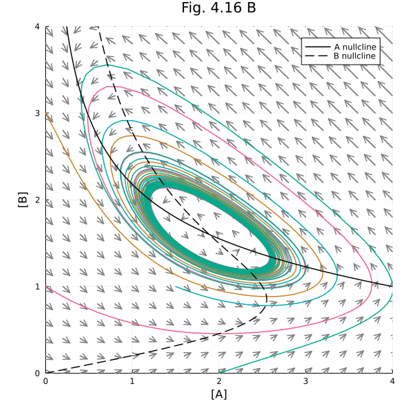

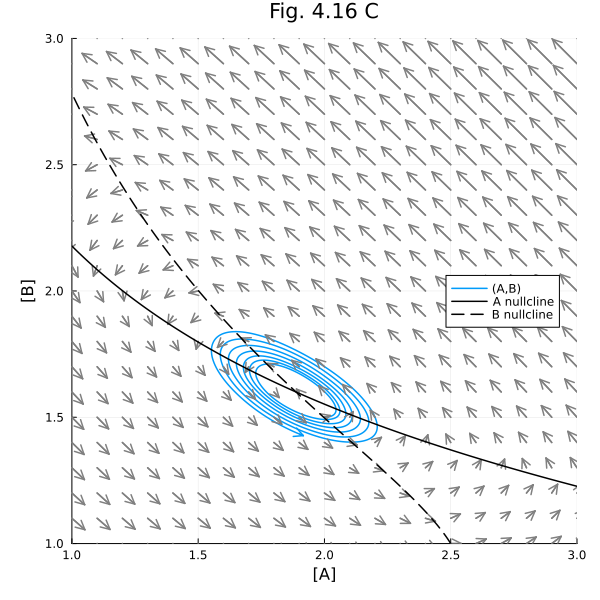
Fig 4.17¶

prob417 = remake(prob416, u0=[:A=>2.0, :B=>1.5], tspan=(0.0, 10.0))
@time sol = solve(prob417, TRBDF2())

plot(sol, idxs=(:A, :B), arrow=(:head))

xrange = range(1, 3, 201)
yrange = range(1, 3, 201)
xx, yy = meshgrid(xrange, yrange)
dx, dy = get_gradient(prob417, :A, :B, xx, yy)
xx_sp = xx[1:10:end, 1:10:end]
yy_sp = yy[1:10:end, 1:10:end]
dx_sp = dx[1:10:end, 1:10:end]
dy_sp = dy[1:10:end, 1:10:end]
dx_sp_norm, dy_sp_norm = normalize_gradient(dx_sp, dy_sp, step(xrange)*10, step(yrange)*10)
quiver!(xx_sp, yy_sp, quiver=(dx_sp_norm, dy_sp_norm), color=:gray)
contour!(xrange, yrange, dx, levels=[0], line=(:black, :solid), colorbar=false)
plot!([], [],  line=(:black, :solid), label="A nullcline")
contour!(xrange, yrange, dy, levels=[0], line=(:black, :dash), colorbar=false)
plot!([], [], line=(:black, :dash), label="B nullcline", legend=:topright)
plot!(title="Fig. 4.16 C", aspect_ratio=1, size=(600, 600), xlims=(1, 3), ylims=(1, 3), xlabel="[A]", ylabel="[B]", legend=:right)

  0.000549 seconds (498 allocations: 37.391 KiB)

Fig 4.18¶

Continuation diagram.

See also BifurcationKit.jl for a more robust continuation diagram.

using SteadyStateDiffEq
using Catalyst
using Plots
Plots.gr(linewidth=1.5)

@time "Build system" model415 = @reaction_network begin
    (k1 / (1 + B^n), k3), 0 <--> A
    k5, A --> B
    (k2, k4), 0 <--> B
end

Build system: 0.000850 seconds (1.52 k allocations: 72.039 KiB)

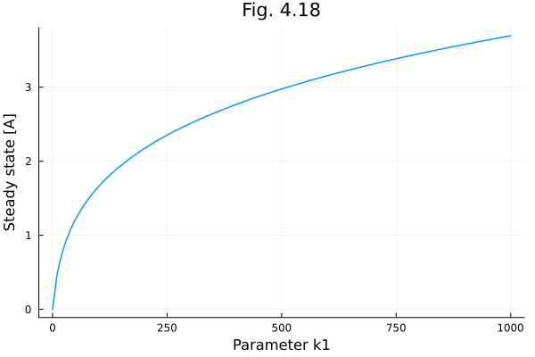
up418 = Dict(:k1 => 0.0, :k2 => 5.0, :k3 => 5.0, :k4 => 5.0, :k5 => 2.0, :n => 4.0, :A => 0.0, :B => 0.0)
@time "Build problem" prob = SteadyStateProblem(model415, up418)

Build problem: 3.977829 seconds (5.60 M allocations: 408.237 MiB, 1.83% gc time, 99.07% compilation time)

SteadyStateProblem with uType Vector{Float64}. In-place: true
u0: 2-element Vector{Float64}:
 0.0
 0.0

k1s = 0.0:10.0:1000.0
prob_func = (prob, i, repeat) -> remake(prob, p=[:k1 => k1s[i]])
output_func=(sol, i) -> (sol[:A], false)
eprob = EnsembleProblem(prob; prob_func, output_func)
alg = DynamicSS(KenCarp47())
@time sim = solve(eprob, alg; trajectories=length(k1s))
plot(k1s, sim.u, xlabel="Parameter k1", ylabel="Steady state [A]", title="Fig. 4.18", label=false)

  7.605261 seconds (12.43 M allocations: 881.434 MiB, 9.08% gc time, 176.36% compilation time)

## Fig 4.22¶

Tangent line.

using Plots
using ForwardDiff

f = x -> 3 / (x-2)
g = x -> ForwardDiff.derivative(f, 4) * (x - 4) + f(4)
plot(f, 2.2, 8.0, label="f(x)")
plot!(g, 2.7, 5.3, label="Tangent line")
plot!(title="Fig. 4.22", xlabel="x", ylabel="f(x)", legend=:topright, xlims=(2, 6), ylims=(0, 5))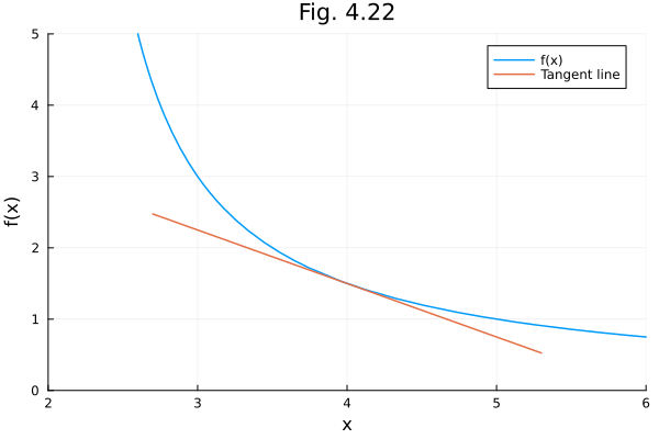

This notebook was generated using Literate.jl.