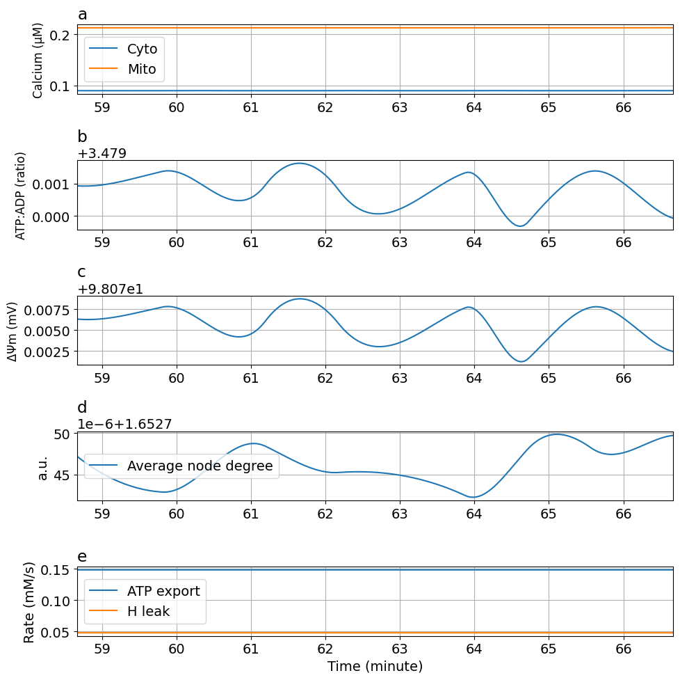
Figure 6: Calcium oscillation#
using OrdinaryDiffEq
using ModelingToolkit
using MitochondrialDynamics
using MitochondrialDynamics: second, μM, mV, mM, Hz, minute, hil
import PythonPlot as plt
plt.matplotlib.rcParams["font.size"] = 14
14
@named sys = make_model()
@unpack Ca_c, Glc, kATPCa, kATP = sys
alg = TRBDF2()
TRBDF2(; linsolve = nothing, nlsolve = OrdinaryDiffEqNonlinearSolve.NLNewton{Rational{Int64}, Rational{Int64}, Rational{Int64}, Nothing}(1//100, 10, 1//5, 1//5, false, true, nothing), precs = DEFAULT_PRECS, smooth_est = true, extrapolant = linear, controller = PI, step_limiter! = trivial_limiter!, autodiff = ADTypes.AutoForwardDiff(),)
Calcium oscillation function
function cac_wave(; ca_base = 0.09μM, ca_act = 0.25μM, n=4, katp=25, amplitude=0.5, period=2minute)
    @variables t Ca_c(t) ATP_c(t) ADP_c(t)
    @parameters (RestingCa=ca_base, ActivatedCa=ca_act, NCac=n, KatpCac=katp)
    x = 5 * ((t / period) % 1.0) ## An oscillating function
    w = (x * exp(1 - x))^4  ## Scale from 0 to 1
    caceq = Ca_c ~ RestingCa + ActivatedCa * hil(ATP_c, KatpCac * ADP_c, NCac) * (1 + amplitude * (2w-1))
    return caceq
end

@named sysosci = make_model(; caceq=cac_wave(amplitude=0.8))

equations(sysosci)

observed(sysosci)
\[\begin{split} \begin{align}
\mathtt{x1}\left( t \right) &= 1 - 3 \mathtt{x3}\left( t \right) - 2 \mathtt{x2}\left( t \right) \\
\mathtt{ATP\_c}\left( t \right) &= \left( \frac{1 - \sqrt{1 + 4 \left( -1 + 4 \mathtt{kEqAK} \right) \mathtt{AEC}\left( t \right) \left( 1 - \mathtt{AEC}\left( t \right) \right)}}{-2 + 8 \mathtt{kEqAK}} + \mathtt{AEC}\left( t \right) \right) \mathtt{{\Sigma}Ac} \\
\mathtt{ADP\_c}\left( t \right) &= \frac{2 \left( -1 + \sqrt{1 + 4 \left( -1 + 4 \mathtt{kEqAK} \right) \mathtt{AEC}\left( t \right) \left( 1 - \mathtt{AEC}\left( t \right) \right)} \right) \mathtt{{\Sigma}Ac}}{-2 + 8 \mathtt{kEqAK}} \\
\mathtt{J\_HL}\left( t \right) &= \mathtt{pHleak} \mathtt{rHL} e^{\mathtt{kvHleak} \mathtt{\Delta{\Psi}m}\left( t \right)} \\
\mathtt{NAD\_c}\left( t \right) &= - \mathtt{NADH\_c}\left( t \right) + \mathtt{{\Sigma}n\_c} \\
\mathtt{NAD\_m}\left( t \right) &= - \mathtt{NADH\_m}\left( t \right) + \mathtt{{\Sigma}n\_m} \\
\mathtt{J\_HR}\left( t \right) &= \frac{\left( 1 + \mathtt{KaETC} \mathtt{\Delta{\Psi}m}\left( t \right) \right) \mathtt{VmaxETC} \mathtt{rETC} \mathtt{NADH\_m}\left( t \right)}{\left( 1 + \mathtt{KbETC} \mathtt{\Delta{\Psi}m}\left( t \right) \right) \left( \mathtt{KnadhETC} + \mathtt{NADH\_m}\left( t \right) \right)} \\
\mathtt{degavg}\left( t \right) &= \frac{3 \mathtt{x3}\left( t \right) + \mathtt{x1}\left( t \right) + 2 \mathtt{x2}\left( t \right)}{\mathtt{x3}\left( t \right) + \mathtt{x1}\left( t \right) + \mathtt{x2}\left( t \right)} \\
\mathtt{J\_GK}\left( t \right) &= \frac{\mathtt{VmaxGK} \mathtt{ATP\_c}\left( t \right) pow\left( \mathtt{Glc}\left( t \right), \mathtt{nGK} \right)}{\left( \mathtt{KatpGK} + \mathtt{ATP\_c}\left( t \right) \right) \left( pow\left( \mathtt{KglcGK}, \mathtt{nGK} \right) + pow\left( \mathtt{Glc}\left( t \right), \mathtt{nGK} \right) \right)} \\
\mathtt{Ca\_c}\left( t \right) &= \mathtt{RestingCa} + \frac{\mathtt{ActivatedCa} \left( 1 + 0.8 \left( -1 + 1250 \left( rem\left( 0.0083333 t, 1 \right) \right)^{4} \left( e^{1 - 5 rem\left( 0.0083333 t, 1 \right)} \right)^{4} \right) \right) pow\left( \mathtt{ATP\_c}\left( t \right), \mathtt{NCac} \right)}{pow\left( \mathtt{KatpCac} \mathtt{ADP\_c}\left( t \right), \mathtt{NCac} \right) + pow\left( \mathtt{ATP\_c}\left( t \right), \mathtt{NCac} \right)} \\
\mathtt{J\_HF}\left( t \right) &= \frac{\mathtt{VmaxF1} \mathtt{rF1} pow\left( \mathtt{FmgadpF1} \mathtt{ADP\_c}\left( t \right), \mathtt{nadpF1} \right) \left( 1 - e^{\frac{ - \mathtt{Ca\_m}\left( t \right)}{\mathtt{KcaF1}}} \right) pow\left( \mathtt{\Delta{\Psi}m}\left( t \right), \mathtt{nvF1} \right)}{\left( pow\left( \mathtt{KvF1}, \mathtt{nvF1} \right) + pow\left( \mathtt{\Delta{\Psi}m}\left( t \right), \mathtt{nvF1} \right) \right) \left( pow\left( \mathtt{KadpF1}, \mathtt{nadpF1} \right) + pow\left( \mathtt{FmgadpF1} \mathtt{ADP\_c}\left( t \right), \mathtt{nadpF1} \right) \right)} \\
\mathtt{AMP\_c}\left( t \right) &= - \mathtt{ATP\_c}\left( t \right) - \mathtt{ADP\_c}\left( t \right) + \mathtt{{\Sigma}Ac} \\
\mathtt{J\_LDH}\left( t \right) &= \frac{\mathtt{VmaxLDH} \mathtt{Pyr}\left( t \right) \mathtt{NADH\_c}\left( t \right)}{\left( \mathtt{NADH\_c}\left( t \right) + \mathtt{KnadhLDH} \mathtt{NAD\_c}\left( t \right) \right) \left( \mathtt{KpyrLDH} + \mathtt{Pyr}\left( t \right) \right)} \\
\mathtt{J\_GPD}\left( t \right) &= \frac{\mathtt{VmaxGPD} \mathtt{NAD\_c}\left( t \right) \mathtt{G3P}\left( t \right) \mathtt{ADP\_c}\left( t \right)}{\left( \mathtt{KadpGPD} + \mathtt{ADP\_c}\left( t \right) \right) \left( \mathtt{Kg3pGPD} + \mathtt{G3P}\left( t \right) \right) \left( \mathtt{NAD\_c}\left( t \right) + \mathtt{KnadGPD} \mathtt{NADH\_c}\left( t \right) \right)} \\
\mathtt{J\_FFA}\left( t \right) &= \mathtt{kFFA} \mathtt{NAD\_m}\left( t \right) \\
\mathtt{J\_PDH}\left( t \right) &= \frac{\mathtt{VmaxPDH} \mathtt{rPDH} \mathtt{NAD\_m}\left( t \right) \mathtt{Pyr}\left( t \right)}{\left( \mathtt{NAD\_m}\left( t \right) + \mathtt{KnadPDH} \mathtt{NADH\_m}\left( t \right) \right) \left( \mathtt{KpyrPDH} + \mathtt{Pyr}\left( t \right) \right) \left( 1 + \left( 1 + \left( \frac{\mathtt{KcaPDH}}{\mathtt{KcaPDH} + \mathtt{Ca\_m}\left( t \right)} \right)^{2} \mathtt{U1PDH} \right) \mathtt{U2PDH} \right)} \\
\mathtt{J\_NADHT}\left( t \right) &= \frac{\mathtt{VmaxNADHT} \mathtt{NAD\_m}\left( t \right) \mathtt{NADH\_c}\left( t \right)}{\left( \mathtt{NADH\_c}\left( t \right) + \mathtt{Ktn\_c} \mathtt{NAD\_c}\left( t \right) \right) \left( \mathtt{NAD\_m}\left( t \right) + \mathtt{Ktn\_m} \mathtt{NADH\_m}\left( t \right) \right)} \\
\mathtt{J\_O2}\left( t \right) &= \frac{1}{10} \mathtt{J\_HR}\left( t \right) \\
\mathtt{J\_MCU}\left( t \right) &= \frac{74.872 \mathtt{PcaMCU} \left( - 0.2 \mathtt{Ca\_m}\left( t \right) + 0.341 \left( 1 + expm1\left( 74.872 \mathtt{\Delta{\Psi}m}\left( t \right) \right) \right) \mathtt{Ca\_c}\left( t \right) \right) \mathtt{\Delta{\Psi}m}\left( t \right)}{expm1\left( 74.872 \mathtt{\Delta{\Psi}m}\left( t \right) \right)} \\
\mathtt{J\_NCLX}\left( t \right) &= \frac{\mathtt{VmaxNCLX} \left( \frac{\left( \frac{\mathtt{Na\_c}}{\mathtt{KnaNCLX}} \right)^{2} \mathtt{Ca\_m}\left( t \right)}{\mathtt{KcaNCLX}} + \frac{ - \left( \frac{\mathtt{Na\_m}}{\mathtt{KnaNCLX}} \right)^{2} \mathtt{Ca\_c}\left( t \right)}{\mathtt{KcaNCLX}} \right)}{1 + \frac{\mathtt{Ca\_m}\left( t \right)}{\mathtt{KcaNCLX}} + \frac{\left( \frac{\mathtt{Na\_c}}{\mathtt{KnaNCLX}} \right)^{2} \mathtt{Ca\_m}\left( t \right)}{\mathtt{KcaNCLX}} + \frac{\mathtt{Ca\_c}\left( t \right)}{\mathtt{KcaNCLX}} + \frac{\left( \frac{\mathtt{Na\_m}}{\mathtt{KnaNCLX}} \right)^{2} \mathtt{Ca\_c}\left( t \right)}{\mathtt{KcaNCLX}} + \left( \frac{\mathtt{Na\_c}}{\mathtt{KnaNCLX}} \right)^{2} + \left( \frac{\mathtt{Na\_m}}{\mathtt{KnaNCLX}} \right)^{2}} \\
\mathtt{J\_ANT}\left( t \right) &= \frac{1}{3} \mathtt{J\_HF}\left( t \right) \\
\mathtt{J\_DH}\left( t \right) &= \mathtt{J\_FFA}\left( t \right) + 4.6 \mathtt{J\_PDH}\left( t \right) \\
\mathtt{tipside}\left( t \right) &= \frac{\mathtt{kfuse2} \mathtt{J\_ANT}\left( t \right) \mathtt{x1}\left( t \right) \mathtt{x2}\left( t \right)}{\mathtt{J\_HL}\left( t \right)} - \mathtt{kfiss2} \mathtt{x3}\left( t \right) \\
\mathtt{tiptip}\left( t \right) &= \frac{\left( \mathtt{x1}\left( t \right) \right)^{2} \mathtt{kfuse1} \mathtt{J\_ANT}\left( t \right)}{\mathtt{J\_HL}\left( t \right)} - \mathtt{kfiss1} \mathtt{x2}\left( t \right)
\end{align}
\end{split}\]
tend = 4000.0
ts = range(tend-480, tend; length=201)
prob = ODEProblem(sysosci, [], tend, [Glc => 10mM])
sol = solve(prob, alg, saveat=ts)
┌ Warning: `SciMLBase.ODEProblem(sys, u0, tspan, p; kw...)` is deprecated. Use
│ `SciMLBase.ODEProblem(sys, merge(if isempty(u0)
│     Dict()
│ else
│     Dict(unknowns(sys) .=> u0)
│ end, Dict(p)), tspan)` instead.
└ @ ModelingToolkit ~/.julia/packages/ModelingToolkit/b28X4/src/deprecations.jl:45
retcode: Success
Interpolation: 1st order linear
t: 201-element Vector{Float64}:
 3520.0
 3522.4
 3524.8
 3527.2
 3529.6
 3532.0
 3534.4
 3536.8
 3539.2
 3541.6
    ⋮
 3980.8
 3983.2
 3985.6
 3988.0
 3990.4
 3992.8
 3995.2
 3997.6
 4000.0
u: 201-element Vector{Vector{Float64}}:
 [0.07298768624306848, 0.24897140514600974, 0.8383275916263325, 0.031581882998430184, 0.0050795153439085715, 0.09807633528770028, 0.0002126738642724931, 0.0028124343488794973, 0.0990545945531673]
 [0.07298765519282241, 0.2489713650818988, 0.8383273436364551, 0.03158186074028627, 0.0050795149774868036, 0.09807630785119426, 0.00021267452146499943, 0.002812433784045538, 0.09905457662206515]
 [0.07298762486822354, 0.24897132715525125, 0.8383272196614614, 0.03158184344107159, 0.005079514778174244, 0.09807628978868912, 0.00021267490775616927, 0.0028124333970135, 0.09905456148956042]
 [0.07298759525189746, 0.2489712913825985, 0.8383272137796624, 0.0315818309354821, 0.005079514738094952, 0.09807628067993325, 0.00021267503526340743, 0.0028124331804523974, 0.09905454908564719]
 [0.07298756632646984, 0.2489712577804719, 0.8383273200693697, 0.03158182305821379, 0.0050795148493729845, 0.09807628010467498, 0.0002126749161041186, 0.0028124331270312475, 0.09905453934031958]
 [0.0729875380745663, 0.2489712263654028, 0.8383275326088949, 0.03158181964396261, 0.005079515104132398, 0.09807628764266269, 0.00021267456239570769, 0.002812433229419066, 0.09905453218357169]
 [0.07298751047881247, 0.2489711971539226, 0.8383278454765496, 0.031581820527424566, 0.005079515494497254, 0.0980763028736447, 0.00021267398625557932, 0.0028124334802848696, 0.09905452754539767]
 [0.07298748352183401, 0.24897117016256273, 0.8383282527506456, 0.03158182554329562, 0.0050795160125916075, 0.09807632537736943, 0.00021267319980113842, 0.0028124338722976742, 0.09905452535579165]
 [0.07298745718625653, 0.24897114540785456, 0.8383287485094942, 0.03158183452627175, 0.005079516650539519, 0.09807635473358522, 0.00021267221514978963, 0.002812434398126496, 0.09905452554474772]
 [0.07298743145470568, 0.24897112290632942, 0.8383293268314069, 0.03158184731104892, 0.005079517400465045, 0.09807639052204042, 0.00021267104441893782, 0.002812435050440352, 0.09905452804226002]
 ⋮
 [0.07298745597949036, 0.24897247623820623, 0.8383007742866869, 0.03158103041201426, 0.005079478820963998, 0.09807399035677364, 0.00021273299604136634, 0.002812396602095271, 0.09905395275351639]
 [0.0729874778352529, 0.24897248777650757, 0.83829739532182, 0.031580831980856615, 0.005079474232119774, 0.09807372554833005, 0.0002127410759094631, 0.002812391220247855, 0.09905384529873096]
 [0.07298750043744294, 0.24897249533203858, 0.838294176034181, 0.03158063364881631, 0.005079469861346299, 0.09807347528175159, 0.00021274886547492853, 0.0028123859971228857, 0.099053738203731]
 [0.07298752361226937, 0.24897249831362886, 0.8382911510573069, 0.03158043705883228, 0.005079465756123401, 0.09807324256173498, 0.00021275628614032864, 0.0028123809832387566, 0.09905363237897294]
 [0.07298754718594118, 0.2489724961301079, 0.8382883550247343, 0.0315802438538435, 0.005079461963930914, 0.09807303039297702, 0.00021276325930822944, 0.002812376229113864, 0.09905352873491322]
 [0.07298757098466731, 0.24897248819030537, 0.8382858225700006, 0.031580055676788926, 0.005079458532248665, 0.0980728417801745, 0.0002127697063811969, 0.002812371785266601, 0.09905342818200817]
 [0.0729875948346567, 0.24897247390305077, 0.8382835883266425, 0.03157987417060751, 0.005079455508556486, 0.09807267972802418, 0.00021277554876179713, 0.0028123677022153636, 0.09905333163071428]
 [0.07298761856211827, 0.24897245267717366, 0.838281686928197, 0.0315797009782382, 0.005079452940334206, 0.09807254724122283, 0.00021278070785259615, 0.0028123640304785454, 0.09905323999148792]
 [0.07298764199326101, 0.24897242392150365, 0.8382801530082011, 0.031579537742619984, 0.005079450875061657, 0.09807244732446721, 0.00021278510505615987, 0.0028123608205745418, 0.09905315417478548]
function plot_fig5(sol, figsize=(10, 10))
    ts = sol.t
    tsm = ts ./ 60
    @unpack Ca_c, Ca_m, ATP_c, ADP_c, ΔΨm, degavg, J_ANT, J_HL = sys
    fig, ax = plt.subplots(5, 1; figsize)

    ax[0].plot(tsm, sol[Ca_c * 1000], label="Cyto")
    ax[0].plot(tsm, sol[Ca_m * 1000], label="Mito")
    ax[0].set_title("a", loc="left")
    ax[0].set_ylabel("Calcium (μM)", fontsize=12)
    ax[0].legend(loc="center left")

    ax[1].plot(tsm, sol[ATP_c / ADP_c])
    ax[1].set_title("b", loc="left")
    ax[1].set_ylabel("ATP:ADP (ratio)", fontsize=12)

    ax[2].plot(tsm, sol[ΔΨm * 1000])
    ax[2].set_title("c", loc="left")
    ax[2].set_ylabel("ΔΨm (mV)", fontsize=12)

    ax[3].plot(tsm, sol[degavg], label="Average node degree")
    ax[3].set_title("d", loc="left")
    ax[3].set_ylabel("a.u.")
    ax[3].legend(loc="center left")

    ax[4].plot(tsm, sol[J_ANT], label="ATP export")
    ax[4].plot(tsm, sol[J_HL], label="H leak")
    ax[4].set_title("e", loc="left")
    ax[4].set_ylabel("Rate (mM/s)")
    ax[4].set(xlabel="Time (minute)")
    ax[4].legend(loc="center left")

    for i in 0:4
        ax[i].grid()
        ax[i].set_xlim(tsm[begin], tsm[end])
    end

    plt.tight_layout()
    return fig
end
plot_fig5 (generic function with 2 methods)
fig5 = plot_fig5(sol)
Export figure
exportTIF(fig5, "Fig6-ca-oscillation.tif")
Python: None
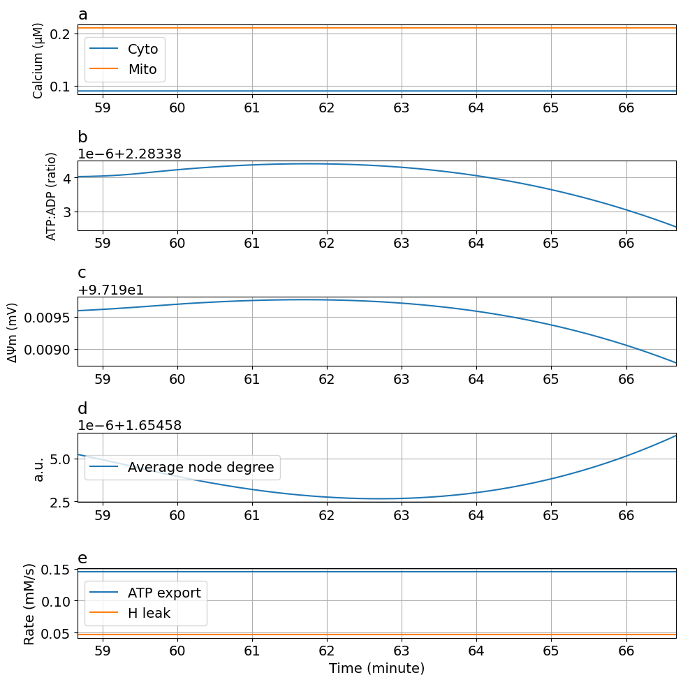
Tuning ca-dependent ATP consumption rate (kATPCa) kATPCa : 90 -> 10
prob2 = ODEProblem(sysosci, [], tend, [Glc => 10mM, kATPCa=>10Hz/mM, kATP=>0.055Hz])
sol2 = solve(prob2, alg, saveat=ts)
plot_fig5(sol2)
┌ Warning: `SciMLBase.ODEProblem(sys, u0, tspan, p; kw...)` is deprecated. Use
│ `SciMLBase.ODEProblem(sys, merge(if isempty(u0)
│     Dict()
│ else
│     Dict(unknowns(sys) .=> u0)
│ end, Dict(p)), tspan)` instead.
└ @ ModelingToolkit ~/.julia/packages/ModelingToolkit/b28X4/src/deprecations.jl:45
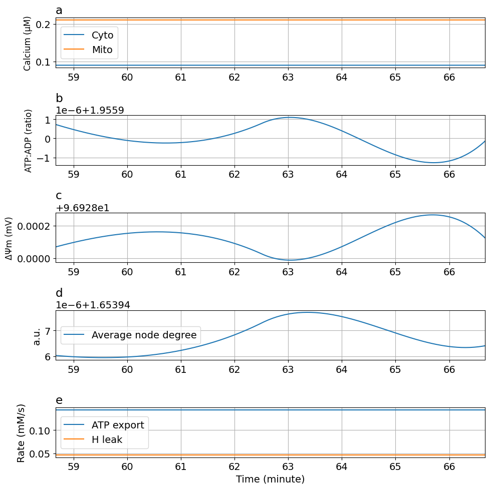
kATPCa : 90 -> 0.1
prob4 = ODEProblem(sysosci, [], tend, [Glc => 10mM, kATPCa=>0.1Hz/mM, kATP=>0.06Hz])
sol4 = solve(prob4, alg, saveat=ts)
plot_fig5(sol4)
┌ Warning: `SciMLBase.ODEProblem(sys, u0, tspan, p; kw...)` is deprecated. Use
│ `SciMLBase.ODEProblem(sys, merge(if isempty(u0)
│     Dict()
│ else
│     Dict(unknowns(sys) .=> u0)
│ end, Dict(p)), tspan)` instead.
└ @ ModelingToolkit ~/.julia/packages/ModelingToolkit/b28X4/src/deprecations.jl:45
This notebook was generated using Literate.jl.