Calcium overload - Mitochondrial dynamics

Steady-state solutions across a range of glucose levels.

using OrdinaryDiffEq
using OrdinaryDiffEqSDIRK
using SteadyStateDiffEq
using ModelingToolkit
using MitochondrialDynamics
using MitochondrialDynamics: μM
import PythonPlot as plt
plt.matplotlib.rcParams["font.size"] = 14

┌ Info: CondaPkg: Waiting for lock to be freed. You may delete this file if no other process is resolving.
└   lock_file = "/home/github/actions-runner-2/_work/mitodyn-ode/mitodyn-ode/.CondaPkg/lock"

14

Default model

@time "Build system" @named sys = make_model()
@time "Build problem" prob = SteadyStateProblem(sys, [])
alg = DynamicSS(TRBDF2())
@time "Solve problem" sol = solve(prob, alg)

Build system: 77.488471 seconds (122.19 M allocations: 6.024 GiB, 4.43% gc time, 99.94% compilation time: 29% of which was recompilation)
Build problem: 30.638438 seconds (60.48 M allocations: 2.995 GiB, 4.29% gc time, 99.78% compilation time: 13% of which was recompilation)
Solve problem: 6.655603 seconds (16.03 M allocations: 806.698 MiB, 2.90% gc time, 99.97% compilation time)

retcode: Success
u: 9-element Vector{Float64}:
 0.05869133954457509
 0.2432316550837996
 0.876502319808825
 0.008756932513658802
 0.002828010003233752
 0.09199008563917664
 0.00020114170980325597
 0.0009825436375669914
 0.057265390364254064

High calcium model

@unpack RestingCa, ActivatedCa = sys
prob_ca5 = SteadyStateProblem(sys, [RestingCa=>0.45μM, ActivatedCa=>1.25μM])
prob_ca10 = SteadyStateProblem(sys, [RestingCa=>0.9μM, ActivatedCa=>2.5μM])

SteadyStateProblem with uType Vector{Float64}. In-place: true
u0: 9-element Vector{Float64}:
 0.06
 0.24
 0.9
 0.0087
 0.0029
 0.092
 0.0002
 0.001
 0.057

Simulating on a range of glucose

@unpack Glc = sys

Model sys:
Equations (9):
  9 standard: see equations(sys)
Unknowns (9): see unknowns(sys)
  x3(t)
  x2(t)
  AEC(t)
  Pyr(t)
  ⋮
Parameters (65): see parameters(sys)
  RestingCa
  NCac
  ActivatedCa
  KatpCac
  ⋮
Observed (24): see observed(sys)

Test on a range of glucose

glc = 3.5:0.5:30.0
prob_func = (prob, ctx) -> begin
    remake(prob, p=[Glc => glc[ctx.sim_id]])
end

trajectories=length(glc)

@time sim = map(glc) do g
    _prob = remake(prob, p=[Glc => g])
    solve(_prob, alg)
end;

@time sim_ca5 = map(glc) do g
    _prob = remake(prob_ca5, p=[Glc => g])
    solve(_prob, alg)
end;

@time sim_ca10 = map(glc) do g
    _prob = remake(prob_ca10, p=[Glc => g])
    solve(_prob, alg)
end;

 13.274394 seconds (22.91 M allocations: 1.114 GiB, 2.15% gc time, 87.83% compilation time: 2% of which was recompilation)
  1.635948 seconds (6.25 M allocations: 300.447 MiB, 5.01% gc time, 6.72% compilation time)
  2.023931 seconds (6.26 M allocations: 301.052 MiB, 27.76% gc time, 5.06% compilation time)

Steady states for a range of glucose¶

function plot_steady_state(glc, sols, sys; figsize=(10, 10), title="")

    @unpack G3P, Pyr, Ca_c, Ca_m, NADH_c, NADH_m, NAD_c, NAD_m, ATP_c, ADP_c, AMP_c, ΔΨm, x1, x2, x3, degavg = sys

    glc5 = glc ./ 5
    g3p = extract(sols, G3P * 1000)
    pyr = extract(sols, Pyr * 1000)
    ca_c = extract(sols, Ca_c * 1000)
    ca_m = extract(sols, Ca_m * 1000)
    nad_ratio_c = extract(sols, NADH_c/NAD_c)
    nad_ratio_m = extract(sols, NADH_m/NAD_m)
    atp_c = extract(sols, ATP_c * 1000)
    adp_c = extract(sols, ADP_c * 1000)
    amp_c = extract(sols, AMP_c * 1000)
    td = extract(sols, ATP_c / ADP_c)
    dpsi = extract(sols, ΔΨm * 1000)
    x1 = extract(sols, x1)
    x2 = extract(sols, x2)
    x3 = extract(sols, x3)
    deg = extract(sols, degavg)

    numrows = 3
    numcols = 3

    fig, ax = plt.subplots(numrows, numcols; figsize)

    ax[0, 0].plot(glc5, g3p)
    ax[0, 0].set(ylabel="G3P (μM)")
    ax[0, 0].set_title("a", loc="left")
    ax[0, 1].plot(glc5, pyr)
    ax[0, 1].set(ylabel="Pyruvate (μM)")
    ax[0, 1].set_title("b", loc="left")
    ax[0, 2].plot(glc5, ca_c, label="cyto")
    ax[0, 2].plot(glc5, ca_m, label="mito")
    ax[0, 2].legend()
    ax[0, 2].set(ylabel="Calcium (μM)")
    ax[0, 2].set_title("c", loc="left")
    ax[1, 0].plot(glc5, nad_ratio_c, label="cyto")
    ax[1, 0].plot(glc5, nad_ratio_m, label="mito")
    ax[1, 0].legend()
    ax[1, 0].set(ylabel="NADH:NAD (ratio)")
    ax[1, 0].set_title("d", loc="left")
    ax[1, 1].plot(glc5, atp_c, label="ATP")
    ax[1, 1].plot(glc5, adp_c, label="ADP")
    ax[1, 1].plot(glc5, amp_c, label="AMP")
    ax[1, 1].legend()
    ax[1, 1].set(ylabel="Adenylates (μM)")
    ax[1, 1].set_title("e", loc="left")
    ax[1, 2].plot(glc5, td)
    ax[1, 2].set(ylabel="ATP:ADP (ratio)")
    ax[1, 2].set_title("f", loc="left")
    ax[2, 0].plot(glc5, dpsi, label="cyto")
    ax[2, 0].set(ylabel="ΔΨ (mV)", xlabel="Glucose (X)")
    ax[2, 0].set_title("g", loc="left")
    ax[2, 1].plot(glc5, x1, label="X1")
    ax[2, 1].plot(glc5, x2, label="X2")
    ax[2, 1].plot(glc5, x3, label="X3")
    ax[2, 1].set(ylabel="Mitochondrial nodes (a.u.)", xlabel="Glucose (X)")
    ax[2, 1].set_title("h", loc="left")
    ax[2, 2].plot(glc5, deg)
    ax[2, 2].set(ylabel="Avg. Node Degree (a.u.)", xlabel="Glucose (X)")
    ax[2, 2].set_title("i", loc="left")

    for i in 0:numrows-1, j in 0:numcols-1
        ax[i, j].set_xticks(1:6)
        ax[i, j].grid()
    end
    fig.suptitle(title)
    fig.tight_layout()
    return fig
end

plot_steady_state (generic function with 1 method)

Default model

fig_glc_default = plot_steady_state(glc, sim, sys, title="Calcium 1X")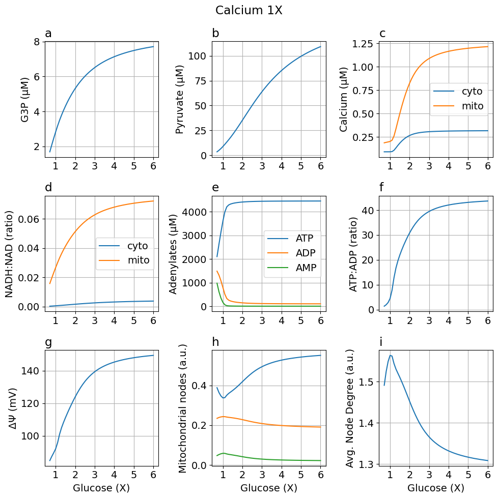

Python: <Figure size 1000x1000 with 9 Axes>

High calcium (5X)

fig_ca5 = plot_steady_state(glc, sim_ca5, sys, title="Calcium 5X")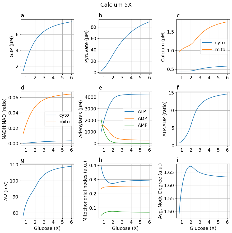

High calcium (10X)

fig_ca10 = plot_steady_state(glc, sim_ca10, sys, title="Calcium 10X")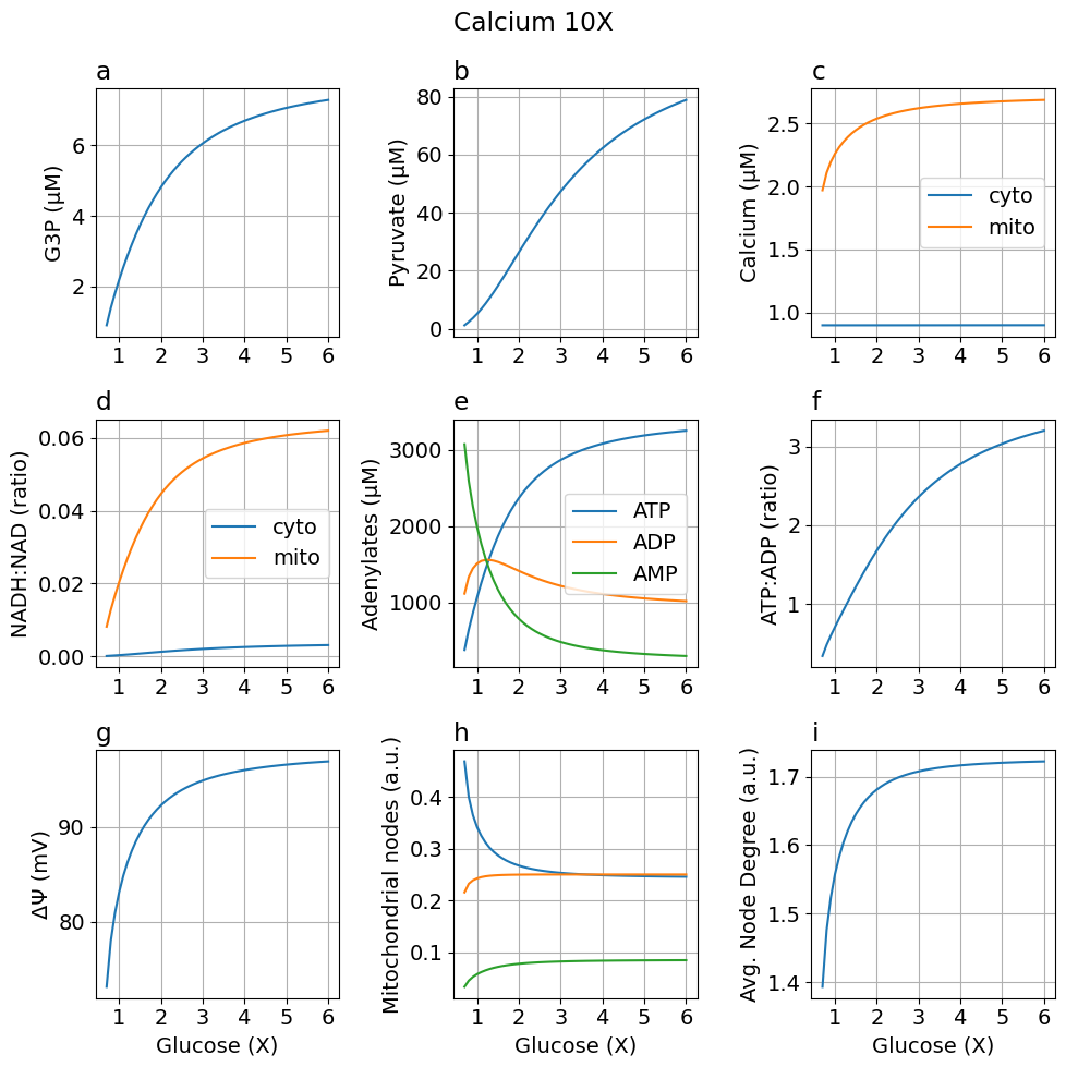

Comparing default and high calcium models¶

function plot_comparision(glc, sim, sim_ca5, sim_ca10, sys;
    figsize=(8, 10), title="", labels=["Ca 1X", "Ca 5X", "Ca 10X"]
)
    @unpack G3P, Pyr, Ca_c, Ca_m, NADH_c, NADH_m, NAD_c, NAD_m, ATP_c, ADP_c, AMP_c, ΔΨm, degavg, J_O2 = sys

    glc5 = glc ./ 5

    numrows = 3
    numcols = 2
    fig, ax = plt.subplots(numrows, numcols; figsize)

    ax[0, 0].set_title("a", loc="left")
    ax[0, 0].set_ylabel("Cyto. NADH:NAD (ratio)")
    k = NADH_c/NAD_c
    yy = [extract(sim, k) extract(sim_ca5, k) extract(sim_ca10, k)]
    lines = ax[0, 0].plot(glc5, yy)
    ax[0, 0].legend(lines, labels)

    ax[0, 1].set_title("b", loc="left")
    ax[0, 1].set_ylabel("Mito. NADH:NAD (ratio)")
    k = NADH_m/NAD_m
    yy = [extract(sim, k) extract(sim_ca5, k) extract(sim_ca10, k)]
    lines = ax[0, 1].plot(glc5, yy)
    ax[0, 1].legend(lines, labels)

    ax[1, 0].set_title("c", loc="left")
    ax[1, 0].set_ylabel("ATP:ADP (ratio)")
    k = ATP_c/ADP_c
    yy = [extract(sim, k) extract(sim_ca5, k) extract(sim_ca10, k)]
    lines = ax[1, 0].plot(glc5, yy)
    ax[1, 0].legend(lines, labels)

    ax[1, 1].set_title("d", loc="left")
    ax[1, 1].set_ylabel("ΔΨm (mV)")
    k = ΔΨm * 1000
    yy = [extract(sim, k) extract(sim_ca5, k) extract(sim_ca10, k)]
    lines = ax[1, 1].plot(glc5, yy)
    ax[1, 1].legend(lines, labels)

    ax[2, 0].set_title("e", loc="left")
    ax[2, 0].set_ylabel("Avg. node degree (ratio)")
    k = degavg
    yy = [extract(sim, k) extract(sim_ca5, k) extract(sim_ca10, k)]
    lines = ax[2, 0].plot(glc5, yy)
    ax[2, 0].legend(lines, labels, loc="lower right")
    ax[2, 0].set(xlabel="Glucose (X)")

    ax[2, 1].set_title("f", loc="left")
    ax[2, 1].set_ylabel("VO2 (mM/s)")
    k = J_O2
    yy = [extract(sim, k) extract(sim_ca5, k) extract(sim_ca10, k)]
    lines = ax[2, 1].plot(glc5, yy)
    ax[2, 1].legend(lines, labels)
    ax[2, 1].set(xlabel="Glucose (X)")

    for i in 0:numrows-1, j in 0:numcols-1
        ax[i, j].set_xticks(1:6)
        ax[i, j].grid()
    end

    fig.suptitle(title)
    fig.tight_layout()
    return fig
end

figcomp = plot_comparision(glc, sim, sim_ca5, sim_ca10, sys)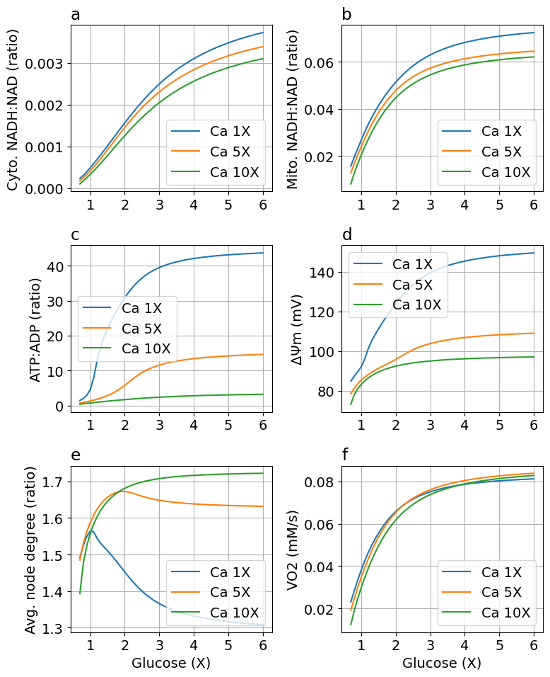

Python: <Figure size 800x1000 with 6 Axes>

Export figure

exportTIF(figcomp, "S1_HighCa.tif")

Python: None

MMP vs ¶

function plot_dpsi_k(sim, sim_ca5, sim_ca10, sys; figsize=(6,6), title="", labels=["Ca 1X", "Ca 5X", "Ca 10X"])
    @unpack ΔΨm, degavg = sys

    fig, ax = plt.subplots(1, 1; figsize)

    ax.plot(extract(sim, ΔΨm * 1000), extract(sim, degavg), "v", label=labels[1])
    ax.plot(extract(sim_ca5, ΔΨm * 1000), extract(sim_ca5, degavg), "o", label=labels[2])
    ax.plot(extract(sim_ca10, ΔΨm * 1000), extract(sim_ca10, degavg), "x", label=labels[3])
    ax.set(xlabel="ΔΨm (mV)", ylabel="Average node degree", title=title)
    ax.legend()
    ax.grid()

    return fig
end

fig = plot_dpsi_k(sim, sim_ca5, sim_ca10, sys)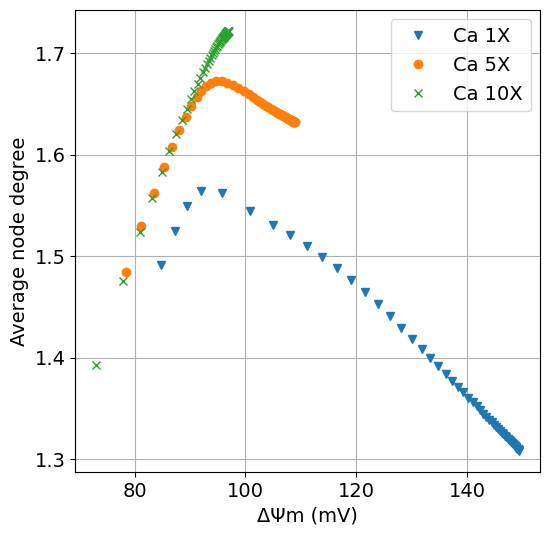

Python: <Figure size 600x600 with 1 Axes>

# exportTIF(fig, "S1_HighCa_dpsi_k.tif")

x-axis as Ca2+ and y-axis as average node degree¶

function plot_ca_k(sim, sim_ca5, sim_ca10, sys; figsize=(6,6), title="", labels=["Ca 1X", "Ca 5X", "Ca 10X"])
    @unpack Ca_m, degavg = sys

    fig, ax = plt.subplots(1, 1; figsize)

    ax.plot(extract(sim, Ca_m * 1000), extract(sim, degavg), "v", label=labels[1])
    ax.plot(extract(sim_ca5, Ca_m * 1000), extract(sim_ca5, degavg), "o", label=labels[2])
    ax.plot(extract(sim_ca10, Ca_m * 1000), extract(sim_ca10, degavg), "x", label=labels[3])
    ax.set(xlabel="Mitochondrial Ca (mM)", ylabel="Average node degree", title=title)
    ax.legend()
    ax.grid()
    return fig
end

fig = plot_ca_k(sim, sim_ca5, sim_ca10, sys)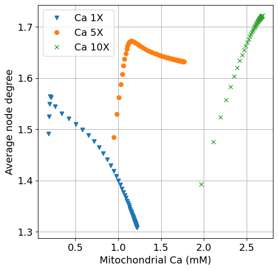

exportTIF(fig, "S1_HighCa_ca_k.tif")

Python: None

x-axis as ATP and y-axis as average node degree¶

function plot_atp_k(sim, sim_ca5, sim_ca10, sys; figsize=(6,6), title="", labels=["Ca 1X", "Ca 5X", "Ca 10X"])
    @unpack ATP_c, ADP_c, degavg = sys

    k = ATP_c / ADP_c

    fig, ax = plt.subplots(1, 1; figsize)

    ax.plot(extract(sim, k), extract(sim, degavg), "v", label=labels[1])
    ax.plot(extract(sim_ca5, k), extract(sim_ca5, degavg), "o", label=labels[2])
    ax.plot(extract(sim_ca10, k), extract(sim_ca10, degavg), "x", label=labels[3])
    ax.set(xlabel="ATP:ADP ratio", ylabel="Average node degree", title=title)
    ax.legend()
    ax.grid()

    return fig
end

fig = plot_atp_k(sim, sim_ca5, sim_ca10, sys)

exportTIF(fig, "S1_HighCa_atp_k.tif")

Python: None

This notebook was generated using Literate.jl.