Chapter 6 - MMSB

Fig 6.3¶

Two component pathway

using Startup

using OrdinaryDiffEq
using Catalyst
using Plots

@time "Build system" rn603 = @reaction_network begin
    @discrete_events begin
        (t == 1.0) => [L => 3.0]
        (t == 3.0) => [L => 0.0]
    end
    (k1 * L, km1), R <--> RL
    k2, RL + P --> RL + Ps
    k3, Ps --> P
end

Build system: 0.636023 seconds (568.63 k allocations: 44.772 MiB, 99.55% compilation time)

up603 = Dict(:k1 => 5.0, :km1 => 1.0, :k2 => 6.0, :k3 => 2.0, :L => 0.0, :R => 3.0, :RL => 0.0, :P => 8.0, :Ps => 0.0)
tend = 10.0
@time "Build problem" prob603 = ODEProblem(rn603, up603, (0.0, tend); remove_conserved=true)
@time "Solve problem" sol603 = solve(prob603, TRBDF2(); tstops=[1.0, 3.0])
plot(sol603, idxs=[:RL, :Ps, :L], labels=["RL" "P*" "L"], title="Fig. 6.3 (A)", xlabel="Time", ylabel="Concentration")

Build problem: 8.227241 seconds (7.58 M allocations: 538.565 MiB, 7.88% gc time, 99.17% compilation time: 11% of which was recompilation)
Solve problem: 4.110406 seconds (6.64 M allocations: 465.081 MiB, 3.46% gc time, 99.87% compilation time)

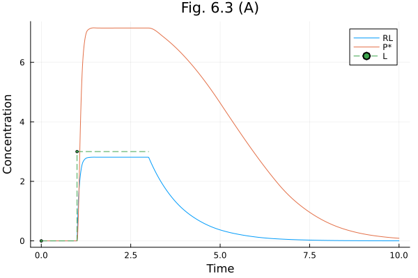
Fig 6.5¶

Model of G-protein signalling pathway

using OrdinaryDiffEq
using SteadyStateDiffEq
using Catalyst
using Plots

@time "Build system" rn605 = @reaction_network begin
    @discrete_events begin
        (t == 200.0) => [L => 1e-9]
        (t == 800.0) => [L => 0.0]
    end
    kRL * L, R --> RL
    kRLm, RL --> R
    kGa, RL + G --> RL + Ga + Gbg
    kGd0, Ga --> Gd
    kG1, Gd + Gbg --> G
end

Build system: 0.001091 seconds (2.57 k allocations: 113.812 KiB)

tend = 1200.0
up605 = Dict(:R => 4e3, :RL => 0.0, :G => 1e4, :Ga => 0.0, :Gd => 0.0, :Gbg => 0.0, :kRL => 2e6, :kRLm => 0.01, :kGa => 1e-5, :kGd0 => 0.11, :kG1 => 1.0, :L => 0.0)
@time "Build problem" prob605 = ODEProblem(rn605, up605, (0.0, tend); remove_conserved=true)
@time "Solve problem" sol = solve(prob605, KenCarp47(); tstops=[200.0, 800.0])
plot(sol, idxs=[:RL, :Ga], labels=["RL" "Ga"], title="Fig. 6.05 (A)", xlabel="Time", ylabel="Concentration")

Build problem: 1.888892 seconds (2.09 M allocations: 149.140 MiB, 2.33% gc time, 96.16% compilation time)
Solve problem: 4.167454 seconds (4.75 M allocations: 329.775 MiB, 2.92% gc time, 99.84% compilation time)

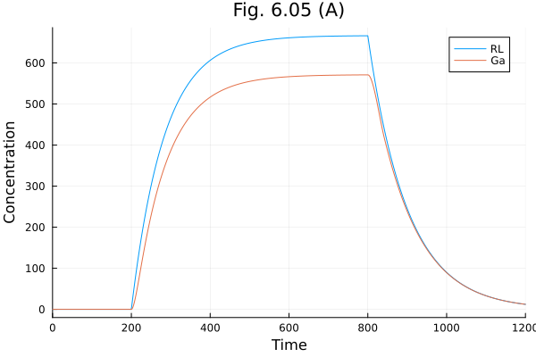
Fig 6.5 B¶

lrange = range(0, 20 * 1e-9, length=101)
@time "Build system" rn605b = @reaction_network begin
    kRL * L, R --> RL
    kRLm, RL --> R
    kGa, RL + G --> RL + Ga + Gbg
    kGd0, Ga --> Gd
    kG1, Gd + Gbg --> G
end

@time "Build problem" prob605b = SteadyStateProblem(rn605b, up605; remove_conserved=true)

@time "Ensemble simulations" sols605 = map(lrange) do lval
    _p = remake(prob605b; p=[:L => lval])
    sol = solve(_p, DynamicSS(KenCarp47()))
end

ga = [sol[:Ga] for sol in sols605]
rl = [sol[:RL] for sol in sols605]
plot(lrange .* 1e9, [ga , rl], label=["Ga" "RL"], xlabel="L (nM)", ylabel="Steady-state abundance", title = "Fig. 6.5 (B)")

Build system: 0.000801 seconds (2.21 k allocations: 102.688 KiB)
Build problem: 4.029097 seconds (5.70 M allocations: 413.792 MiB, 2.48% gc time, 98.86% compilation time)
Ensemble simulations: 7.795655 seconds (14.32 M allocations: 930.172 MiB, 3.47% gc time, 85.34% compilation time)

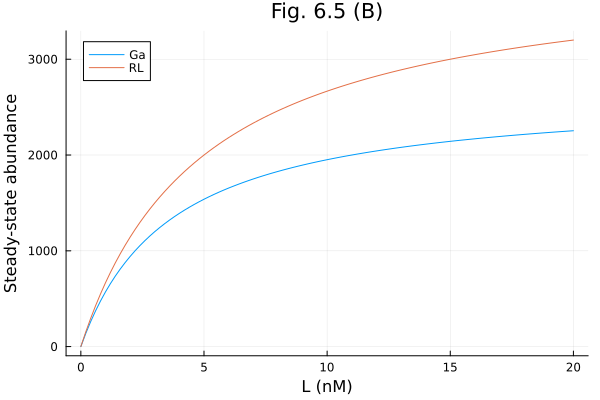
Fig 6.07¶

Goldbeter Koshland switch

using Plots
f607(w, K1, K2) = w * (1 - w + K1)/((1 - w) * (w + K2))
yy = 0:0.001:0.999
xx1 = f607.(yy, 1, 1)
xx2 = f607.(yy, 0.1, 0.1)
xx3 = f607.(yy, 0.01, 0.01)

plot(xx1, yy, label="K1=K2=1", xlabel="Stimulus", ylabel="Response", title="Fig 6.07", xlims=(0, 3), ylims=(0, 1))
plot!(xx2, yy, label="K1=K2=0.1")
plot!(xx3, yy, label="K1=K2=0.01")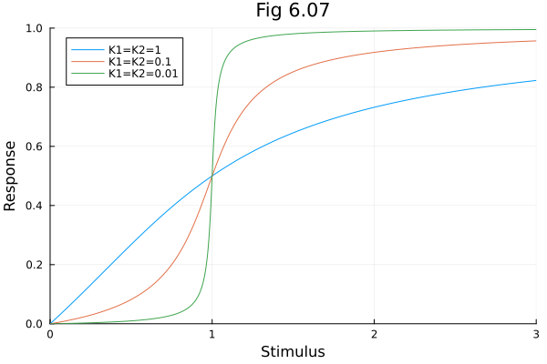

Fig 6.14¶

Model of E. coli chemotaxis signalling pathway

using OrdinaryDiffEq
using Catalyst
using Plots

@time "Build system" rn614 = @reaction_network begin
    @discrete_events begin
        (t == 10.0) => [L => 40.0]
        (t == 30.0) => [L => 80.0]
    end
    mm(Am, k1 * BP, KM1), Am => A
    mm(AmL, k2 * BP, KM2), AmL => AL
    km1 * R , A => Am
    km2 * R , AL => AmL
    (k3 * L, km3), Am <--> AmL
    (k4 * L, km4), A <--> AL
    (k5 * Am, km5), B <--> BP
end

Build system: 0.060933 seconds (171.83 k allocations: 12.101 MiB, 97.55% compilation time)

up614 = Dict(
    :Am => 0.0360,
    :AmL => 1.5593,
    :A => 0.0595,
    :AL => 0.3504,
    :B => 0.7356,
    :BP => 0.2644,
    :k1 => 200.0,
    :k2 => 1.0,
    :k3 => 1.0,
    :km1 => 1.0,
    :km2 => 1.0,
    :km3 => 1.0,
    :k4 => 1.0,
    :km4 => 1.0,
    :k5 => 0.05,
    :km5 => 0.005,
    :KM1 => 1.0,
    :KM2 => 1.0,
    :L => 20.0,
    :R => 1.0,
)

tend = 50.0
@time "Build problem" prob614 = ODEProblem(rn614, up614, (0.0, tend); remove_conserved=true)
@time "Solve problem" sol614 = solve(prob614, FBDF(); tstops=[10.0, 30.0])
plot(sol614, idxs=[:Am], title="Fig 6.14", xlabel="Time", ylabel="Concentration")

Build problem: 1.421028 seconds (2.12 M allocations: 151.703 MiB, 2.15% gc time, 96.10% compilation time)
Solve problem: 4.166260 seconds (4.58 M allocations: 315.781 MiB, 2.81% gc time, 99.85% compilation time)

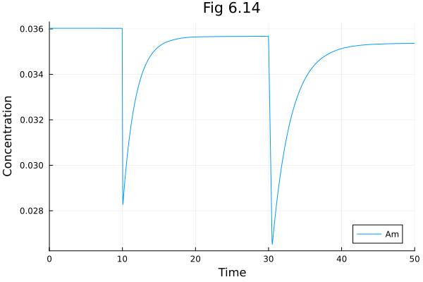
Fig 6.16¶

Model of apoptosis signalling pathway

using Catalyst
using OrdinaryDiffEq
using Plots

@time "Build system" rn616 = @reaction_network begin
    @discrete_events begin
        (t == 100.0) => [I => 200.0]
        (t == 1200.0) => [I => 0.0]
    end
    (k1, k2), 0 <--> C8
    k3 * (C3s + I), C8 --> C8s
    k4, C8s --> 0
    (k5, k6), C8s + BAR <--> C8sBAR
    (k7, k8), 0 <--> C3
    k9 * C8s, C3 --> C3s
    k10, C3s --> 0
    (k11, k12), C3s + IAP <--> C3sIAP
    (k13, k14), 0 <--> BAR
    (k15, k16 + k17 * C3s), 0 <--> IAP
    k18, C8sBAR --> 0
    k19, C3sIAP --> 0
end

Build system: 0.001457 seconds (5.44 k allocations: 233.219 KiB)

up616 = Dict(
    :C8 => 1.3E5,
    :C8s => 0.0,
    :C3 => 0.21E5,
    :C3s => 0.0,
    :BAR => 0.4E5,
    :IAP => 0.4E5,
    :C8sBAR => 0.0,
    :C3sIAP => 0.0,
    :k1 => 507.0,
    :k2 => 3.9e-3,
    :k3 => 1e-5,
    :k4 => 5.8e-3,
    :k5 => 5e-4,
    :k6 => 0.21,
    :k7 => 81.9,
    :k8 => 3.9e-3,
    :k9 => 5.8e-6,
    :k10 => 5.8e-3,
    :k11 => 5e-4,
    :k12 => 0.21,
    :k13 => 40.0,
    :k14 => 1e-3,
    :k15 => 464.0,
    :k16 => 1.16e-2,
    :k17 => 3e-4,
    :k18 => 1.16e-2,
    :k19 => 1.73e-2,
    :I => 0.0,
)

tend = 1800.0
@time "Build problem" prob616 = ODEProblem(rn616, up616, (0.0, tend); remove_conserved=true)
@time "Solve problem" sol616 = solve(prob616, FBDF(); tstops=[100.0, 1200.0])


@unpack C3s, C8s, I = rn616
plot(sol616, idxs=[C3s, C8s, I*100], title="Fig 6.16", xlabel="Time", ylabel="Concentration", legend=:right)

Build problem: 1.060038 seconds (1.34 M allocations: 97.282 MiB, 3.28% gc time, 95.28% compilation time)
Solve problem: 3.158107 seconds (3.90 M allocations: 269.380 MiB, 1.39% gc time, 99.82% compilation time)

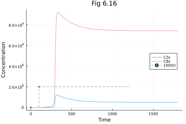
Fig 6.18¶

Model of calcium-induced calcium release in hepatocytes

using Catalyst
using OrdinaryDiffEq
using Plots

@time "Build system" rn618 = @reaction_network begin
    @discretes I(t)
    (k1 * I, km1), R <--> RI
    (k2 * C, km2), RI <--> RIC
    (k3 * C, km3), RIC <--> RICC
    vr * (γ0 + γ1 * RIC) * (Cer - C), 0 --> C
    hill(C, p1, p2, 4), C => 0
end

Build system: 0.329531 seconds (329.02 k allocations: 23.468 MiB, 9.89% gc time, 99.46% compilation time)

up618 = Dict(
    :C => 0.0,
    :R => 1.0,
    :RI => 0.0,
    :RIC => 0.0,
    :RICC => 0.0,
    :k1 => 12.0,
    :km1 => 8.0,
    :k2 => 15.0,
    :km2 => 1.65,
    :k3 => 1.8,
    :km3 => 0.21,
    :vr => 0.185,
    :γ0 => 0.1,
    :γ1 => 20.5,
    :p1 => 8.5,
    :p2 => 0.065,
    :Cer => 8.37,
    :I => 0.0
)

Dict{Symbol, Float64} with 18 entries:
  :RI   => 0.0
  :RIC  => 0.0
  :R    => 1.0
  :p2   => 0.065
  :k1   => 12.0
  :km3  => 0.21
  :k3   => 1.8
  :vr   => 0.185
  :γ0   => 0.1
  :γ1   => 20.5
  :p1   => 8.5
  :I    => 0.0
  :Cer  => 8.37
  :RICC => 0.0
  :km1  => 8.0
  :k2   => 15.0
  :km2  => 1.65
  :C    => 0.0

Fig 6.18 (A)¶

tspan = (0.0, 25.0)
up618a = merge(up618, Dict(:I => 2.0))
@time "Build problem" prob618a = ODEProblem(rn618, up618a, tspan; remove_conserved=true)
@time "Solve problem" sol618a = solve(prob618a, KenCarp47())
plot(sol618a, idxs=[:C, :RIC, :RICC], title="Fig 6.18 (A)", xlabel="Time", ylabel="Abundance", legend=:topright)

Build problem: 1.186991 seconds (1.86 M allocations: 133.780 MiB, 5.18% gc time, 96.14% compilation time)
Solve problem: 2.600075 seconds (3.73 M allocations: 258.833 MiB, 2.58% gc time, 99.79% compilation time)

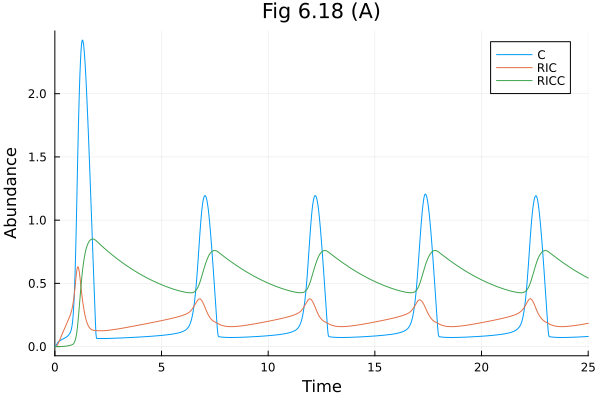
Fig 6.18 (B)¶

@unpack I = rn618
events = [
    ModelingToolkitBase.SymbolicDiscreteCallback([20.0] => [I ~ 0.7]; discrete_parameters=[I]),
    ModelingToolkitBase.SymbolicDiscreteCallback([60.0] => [I ~ 1.2]; discrete_parameters=[I]),
    ModelingToolkitBase.SymbolicDiscreteCallback([90.0] => [I ~ 4.0]; discrete_parameters=[I])
]

osys618 = ode_model(rn618; remove_conserved=true, discrete_events=events)
tend = 120.0
prob618b = ODEProblem(osys618 |> complete, up618, tend)
@time sol618b = solve(prob618b, KenCarp47())
plot(sol618b, idxs=[:C], title="Fig 6.18 (B)", label="Calcium", xlabel="Time", ylabel="Concentration", legend=:topright)

  3.969967 seconds (5.07 M allocations: 346.046 MiB, 2.01% gc time, 99.78% compilation time)

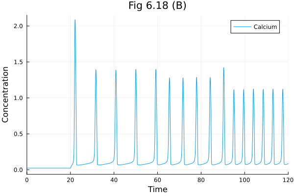
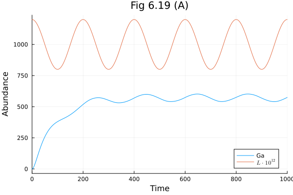
Fig 6.19¶

Sine wave response of g-protein signalling pathway

using OrdinaryDiffEq
using Catalyst
using Plots
using LaTeXStrings

@time "Build system" rn605 = @reaction_network begin
    @parameters lt l_AMP l_per
    @equations begin
        L ~ lt + (lt / l_AMP) * cospi(2t / l_per)
    end
    kRL * L, R --> RL
    kRLm, RL --> R
    kGa, RL + G --> RL + Ga + Gbg
    kGd0, Ga --> Gd
    kG1, Gd + Gbg --> G
end

Build system: 0.117919 seconds (203.43 k allocations: 14.331 MiB, 98.30% compilation time: 12% of which was recompilation)

up619 = Dict(
    :kRL => 2e6,
    :kRLm => 0.01,
    :kGa => 1e-5,
    :kGd0 => 0.11,
    :kG1 => 1.0,
    :R => 4e3,
    :G => 1e4,
    :lt => 1e-9,
    :l_per => 200.0,
    :l_AMP => 5.0,
    :RL => 0.0,
    :Ga => 0.0,
    :Gd => 0.0,
    :Gbg => 0.0
)

tend = 1000.0
@time "Build problem" prob619 = ODEProblem(rn605, up619, (0.0, tend); mtkcompile=true)
@time "Solve problem" sol619 = solve(prob619, KenCarp47())

@unpack Ga, L = rn605
plot(sol619, idxs=[Ga, L*1E12], title="Fig 6.19 (A)", xlabel="Time", ylabel="Abundance", label=["Ga" L"L \cdot 10^{12}"])

Build problem: 0.773562 seconds (1.11 M allocations: 81.469 MiB, 4.23% gc time, 94.83% compilation time)
Solve problem: 0.649130 seconds (948.06 k allocations: 66.660 MiB, 99.43% compilation time)

This notebook was generated using Literate.jl.