using OrdinaryDiffEq
using SteadyStateDiffEq
using DiffEqCallbacks
using Catalyst
using Plots
Plots.gr(linewidth=1.5)Plots.GRBackend()Convenience functions to plot gradients of the ODEs.
function meshgrid(xrange, yrange)
    xx = [x for y in yrange, x in xrange]
    yy = [y for y in yrange, x in xrange]
    return xx, yy
end

"Get the gradients of the vector field of an ODE system at a grid of points in the state space."
function get_gradient(prob, xsym, ysym, xx, yy; t = nothing)
    # The order of state variables (unknowns) in the ODE system is not guaranteed. So we may need to swap the order of x and y when calling ∂F.
    swap_or_not(x, y; xidx=1) = xidx == 1 ? [x, y] : [y, x]
    ∂F = prob.f
    ps = prob.p
    sys = prob.f.sys
    xidx = ModelingToolkit.variable_index(sys, xsym)
    yidx = ModelingToolkit.variable_index(sys, ysym)
    dx = map((x, y) -> ∂F(swap_or_not(x, y; xidx), ps, t)[xidx], xx, yy)
    dy = map((x, y) -> ∂F(swap_or_not(x, y; xidx), ps, t)[yidx], xx, yy)
    return (dx, dy)
end

function normalize_gradient(dx, dy, xscale, yscale; transform=cbrt)
    maxdx = maximum(abs, dx)
    maxdy = maximum(abs, dy)
    dx_norm = @. transform(dx / maxdx) * xscale
    dy_norm = @. transform(dy / maxdy) * yscale
    return (dx_norm, dy_norm)
end
normalize_gradient (generic function with 1 method)Fig 7.7
Model of lac operon in E. coli.
@time "Build system" rn707 = @reaction_network begin
    (a1 / (1 + RToverK1 * (K2 / (K2 + L))^4), δM), 0 <--> M
    (c1 * M, δY), 0 <--> Y
    mm(Le, kL * Y, KML), 0 --> L
    δL, L --> 0
    (Y/4) * mm(L, 2kg, KMg), L => 0
end
Build system: 18.441514 seconds (43.11 M allocations: 2.115 GiB, 2.26% gc time, 99.95% compilation time: 14% of which was recompilation)
Loading...
up707 = Dict(
    :δM => 0.48, :δY => 0.03, :δL => 0.02,
    :a1 => 0.29,:K2 => 2.92e6, :RToverK1 => 213.2, :c1 => 18.8,
    :kL => 6e4, :KML => 680.0, :kg => 3.6e3, :KMg => 7e5,
    :Le => 0.0, :M => 0.01, :Y => 0.1, :L => 0.0,
)

@unpack Le = rn707
cbs = let
    event_le1 = PresetTimeCallback([500.0], (integrator) -> integrator.ps[Le] = 50)
    event_le2 = PresetTimeCallback([1000.0], (integrator) -> integrator.ps[Le] = 100)
    event_le3 = PresetTimeCallback([1500.0], (integrator) -> integrator.ps[Le] = 150)
    event_le4 = PresetTimeCallback([2000.0], (integrator) -> integrator.ps[Le] = 0)
    CallbackSet(event_le1, event_le2, event_le3, event_le4)
end
SciMLBase.CallbackSet{Tuple{}, Tuple{SciMLBase.DiscreteCallback{DiffEqCallbacks.PresetTimeFunction{Vector{Float64}, typeof(SciMLBase.INITIALIZE_DEFAULT), Main.var"##277".var"#18#19"}, Main.var"##277".var"#18#19", DiffEqCallbacks.PresetTimeFunction{Vector{Float64}, typeof(SciMLBase.INITIALIZE_DEFAULT), Main.var"##277".var"#18#19"}, typeof(SciMLBase.FINALIZE_DEFAULT), Nothing, Tuple{}}, SciMLBase.DiscreteCallback{DiffEqCallbacks.PresetTimeFunction{Vector{Float64}, typeof(SciMLBase.INITIALIZE_DEFAULT), Main.var"##277".var"#20#21"}, Main.var"##277".var"#20#21", DiffEqCallbacks.PresetTimeFunction{Vector{Float64}, typeof(SciMLBase.INITIALIZE_DEFAULT), Main.var"##277".var"#20#21"}, typeof(SciMLBase.FINALIZE_DEFAULT), Nothing, Tuple{}}, SciMLBase.DiscreteCallback{DiffEqCallbacks.PresetTimeFunction{Vector{Float64}, typeof(SciMLBase.INITIALIZE_DEFAULT), Main.var"##277".var"#22#23"}, Main.var"##277".var"#22#23", DiffEqCallbacks.PresetTimeFunction{Vector{Float64}, typeof(SciMLBase.INITIALIZE_DEFAULT), Main.var"##277".var"#22#23"}, typeof(SciMLBase.FINALIZE_DEFAULT), Nothing, Tuple{}}, SciMLBase.DiscreteCallback{DiffEqCallbacks.PresetTimeFunction{Vector{Float64}, typeof(SciMLBase.INITIALIZE_DEFAULT), Main.var"##277".var"#24#25"}, Main.var"##277".var"#24#25", DiffEqCallbacks.PresetTimeFunction{Vector{Float64}, typeof(SciMLBase.INITIALIZE_DEFAULT), Main.var"##277".var"#24#25"}, typeof(SciMLBase.FINALIZE_DEFAULT), Nothing, Tuple{}}}}((), (SciMLBase.DiscreteCallback{DiffEqCallbacks.PresetTimeFunction{Vector{Float64}, typeof(SciMLBase.INITIALIZE_DEFAULT), Main.var"##277".var"#18#19"}, Main.var"##277".var"#18#19", DiffEqCallbacks.PresetTimeFunction{Vector{Float64}, typeof(SciMLBase.INITIALIZE_DEFAULT), Main.var"##277".var"#18#19"}, typeof(SciMLBase.FINALIZE_DEFAULT), Nothing, Tuple{}}(DiffEqCallbacks.PresetTimeFunction{Vector{Float64}, typeof(SciMLBase.INITIALIZE_DEFAULT), Main.var"##277".var"#18#19"}([500.0], true, SciMLBase.INITIALIZE_DEFAULT, Main.var"##277".var"#18#19"()), Main.var"##277".var"#18#19"(), DiffEqCallbacks.PresetTimeFunction{Vector{Float64}, typeof(SciMLBase.INITIALIZE_DEFAULT), Main.var"##277".var"#18#19"}([500.0], true, SciMLBase.INITIALIZE_DEFAULT, Main.var"##277".var"#18#19"()), SciMLBase.FINALIZE_DEFAULT, Bool[1, 1], nothing, (), true), SciMLBase.DiscreteCallback{DiffEqCallbacks.PresetTimeFunction{Vector{Float64}, typeof(SciMLBase.INITIALIZE_DEFAULT), Main.var"##277".var"#20#21"}, Main.var"##277".var"#20#21", DiffEqCallbacks.PresetTimeFunction{Vector{Float64}, typeof(SciMLBase.INITIALIZE_DEFAULT), Main.var"##277".var"#20#21"}, typeof(SciMLBase.FINALIZE_DEFAULT), Nothing, Tuple{}}(DiffEqCallbacks.PresetTimeFunction{Vector{Float64}, typeof(SciMLBase.INITIALIZE_DEFAULT), Main.var"##277".var"#20#21"}([1000.0], true, SciMLBase.INITIALIZE_DEFAULT, Main.var"##277".var"#20#21"()), Main.var"##277".var"#20#21"(), DiffEqCallbacks.PresetTimeFunction{Vector{Float64}, typeof(SciMLBase.INITIALIZE_DEFAULT), Main.var"##277".var"#20#21"}([1000.0], true, SciMLBase.INITIALIZE_DEFAULT, Main.var"##277".var"#20#21"()), SciMLBase.FINALIZE_DEFAULT, Bool[1, 1], nothing, (), true), SciMLBase.DiscreteCallback{DiffEqCallbacks.PresetTimeFunction{Vector{Float64}, typeof(SciMLBase.INITIALIZE_DEFAULT), Main.var"##277".var"#22#23"}, Main.var"##277".var"#22#23", DiffEqCallbacks.PresetTimeFunction{Vector{Float64}, typeof(SciMLBase.INITIALIZE_DEFAULT), Main.var"##277".var"#22#23"}, typeof(SciMLBase.FINALIZE_DEFAULT), Nothing, Tuple{}}(DiffEqCallbacks.PresetTimeFunction{Vector{Float64}, typeof(SciMLBase.INITIALIZE_DEFAULT), Main.var"##277".var"#22#23"}([1500.0], true, SciMLBase.INITIALIZE_DEFAULT, Main.var"##277".var"#22#23"()), Main.var"##277".var"#22#23"(), DiffEqCallbacks.PresetTimeFunction{Vector{Float64}, typeof(SciMLBase.INITIALIZE_DEFAULT), Main.var"##277".var"#22#23"}([1500.0], true, SciMLBase.INITIALIZE_DEFAULT, Main.var"##277".var"#22#23"()), SciMLBase.FINALIZE_DEFAULT, Bool[1, 1], nothing, (), true), SciMLBase.DiscreteCallback{DiffEqCallbacks.PresetTimeFunction{Vector{Float64}, typeof(SciMLBase.INITIALIZE_DEFAULT), Main.var"##277".var"#24#25"}, Main.var"##277".var"#24#25", DiffEqCallbacks.PresetTimeFunction{Vector{Float64}, typeof(SciMLBase.INITIALIZE_DEFAULT), Main.var"##277".var"#24#25"}, typeof(SciMLBase.FINALIZE_DEFAULT), Nothing, Tuple{}}(DiffEqCallbacks.PresetTimeFunction{Vector{Float64}, typeof(SciMLBase.INITIALIZE_DEFAULT), Main.var"##277".var"#24#25"}([2000.0], true, SciMLBase.INITIALIZE_DEFAULT, Main.var"##277".var"#24#25"()), Main.var"##277".var"#24#25"(), DiffEqCallbacks.PresetTimeFunction{Vector{Float64}, typeof(SciMLBase.INITIALIZE_DEFAULT), Main.var"##277".var"#24#25"}([2000.0], true, SciMLBase.INITIALIZE_DEFAULT, Main.var"##277".var"#24#25"()), SciMLBase.FINALIZE_DEFAULT, Bool[1, 1], nothing, (), true)))Fig 7.07 (A)
tend = 2500.0
@time "Build problem" prob707a = ODEProblem(rn707, up707, tend)
@time "Solve problem" sol = solve(prob707a, KenCarp47(), callback=cbs)

plot(sol, idxs=[:Y], labels="β-galactosidase monomer", title="Fig 7.07 (A)", xlabel="Time (min)", ylabel="Concentration")
plot!(t -> 50 * (500<=t<1000) + 100 * (1000<=t<1500) + 150 * (1500<=t<2000), 0, tend, linestyle=:dash, label="External lactose")
Build problem: 40.064800 seconds (76.99 M allocations: 3.790 GiB, 1.53% gc time, 99.89% compilation time: 51% of which was recompilation)
Solve problem: 4.610335 seconds (10.30 M allocations: 528.762 MiB, 0.98% gc time, 99.83% compilation time)
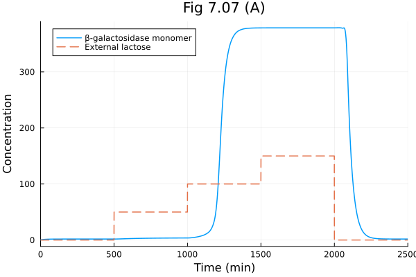
Fig 7.07 (B)
Comparing the original model and the modified model
@time "Build system" rn707b = @reaction_network begin
    (a1 / (1 + RToverK1 * (K2 / (K2 + L))^4), δM), 0 <--> M
    (c1 * M, δY), 0 <--> Y
    Enz * mm(Le, 4kL, KML), 0 --> L
    δL, L --> 0
    Enz * mm(L, 2kg, KMg), L => 0
end
Build system: 0.001025 seconds (2.84 k allocations: 105.875 KiB)
Loading...
up707b = merge(up707, Dict(:Enz => 40.0))
prob707a = SteadyStateProblem(rn707, up707)
prob707b = SteadyStateProblem(rn707b, up707b)
lerange = 0:100
prob_func = (prob, i, repeat) -> remake(prob, p=[:Le => lerange[i]])
output_func=(sol, i) -> (sol[:Y] / 4, false)
alg = DynamicSS(KenCarp47())

eprob = EnsembleProblem(prob707a; prob_func, output_func)
eprob_mod = EnsembleProblem(prob707b; prob_func, output_func)
@time sim = solve(eprob, alg; trajectories=length(lerange))
@time sim_mod = solve(eprob_mod, alg; trajectories=length(lerange))

plot(lerange, [sim.u sim_mod.u], labels=["Original model" "Modified model"], title="Fig 7.07 (B)", xlabel="External lactose concentration", ylabel="β-galactosidase tetramer concentration")
10.506051 seconds (26.27 M allocations: 1.356 GiB, 4.59% gc time, 22066 lock conflicts, 358.92% compilation time)
4.440244 seconds (12.25 M allocations: 694.749 MiB, 1.65% gc time, 25944 lock conflicts, 329.97% compilation time)
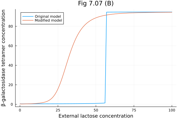
Fig 7.11
Model of phage lambda decision switch
using ModelingToolkit
using ModelingToolkit: t_nounits as t, D_nounits as D
using OrdinaryDiffEq
using Plots
function build_sys711(; name=:model711, simplify=true)
@parameters K1=1 K2=0.1 K3=5 K4=0.5 delta_r=0.02 delta_c=0.02 a=5 b=50
@variables r(t)=0 c(t)=0 rd(t) cd(t)
rd = r / 2
cd = c / 2
f1 = K1 * rd^2
f2 = K2 * rd
f3 = K3 * cd
f4 = K4 * cd
den = 1 + f1 * (1 + f2) + f3 * (1 + f4)
Dr = a * (1 + 10 * f1) / den - delta_r * r
Dc = b * (1 + f3) / den - delta_c * c
eqs = [
D(r) ~ Dr,
D(c) ~ Dc
]
sys = ODESystem(eqs, t; name)
return simplify ? mtkcompile(sys) : sys
endbuild_sys711 (generic function with 1 method)@time "Build system" sys711 = build_sys711()
@time "Build problem" prob711 = ODEProblem(sys711, [], (0.0, 6000.0))Build system: 16.974543 seconds (18.63 M allocations: 915.817 MiB, 0.59% gc time, 99.90% compilation time: 65% of which was recompilation)
Build problem: 10.496753 seconds (28.00 M allocations: 1.397 GiB, 3.98% gc time, 99.74% compilation time: 69% of which was recompilation)
ODEProblem with uType Vector{Float64} and tType Float64. In-place: true
Initialization status: FULLY_DETERMINED
Non-trivial mass matrix: false
timespan: (0.0, 6000.0)
u0: 2-element Vector{Float64}:
 0.0
 0.0
xrange = range(0, 250, 101)
yrange = range(0, 250, 101)
@unpack r, c, delta_r = sys711
xx, yy = meshgrid(xrange, yrange)
dx, dy = get_gradient(prob711, r, c, xx, yy)
xx_sp = xx[1:5:end, 1:5:end]
yy_sp = yy[1:5:end, 1:5:end]
dxnorm, dynorm = normalize_gradient(dx[1:5:end, 1:5:end], dy[1:5:end, 1:5:end], 5*step(xrange), 5*step(yrange))([6.869900720736457 12.5 … -3.830155728956546 -4.380542181421769; 1.3564603768501013 8.619503079010805 … -3.8342111861666335 -4.383088669865122; … ; 0.2083496781398712 -2.33161695290965 … -4.605918652952202 -4.917933080036901; 0.20140128284987327 -2.352372751490533 … -4.662569067589072 -4.9609030705045996], [12.5 3.117281732278567 … 0.2207518698458821 0.20998650981913586; 7.803052086269383 6.81094309069183 … -2.111870814296849 -2.1154713520348527; … ; -5.350151664320803 -5.3508185574376315 … -5.648346145868846 -5.654984302895317; -5.479329459661966 -5.4798755632023 … -5.746740666493403 -5.75327189248827])quiver(xx_sp, yy_sp, quiver=(dxnorm, dynorm); aspect_ratio=1, size=(600, 600), xlims=(0, 250), ylims=(0, 250), color=:gray)
contour!(xrange, yrange, dx, levels=[0], line=(:black, :solid), colorbar=false)
plot!([], [], line=(:black, :solid), label="R nullcline")
contour!(xrange, yrange, dy, levels=[0], line=(:black, :dash), colorbar=false)
plot!([], [], line=(:black, :dash), label="C nullcline")
plot!(xlabel="[cI] (nM)", ylabel="[cro] (nM)", title="Fig. 7.11 (A)", legend=:topright)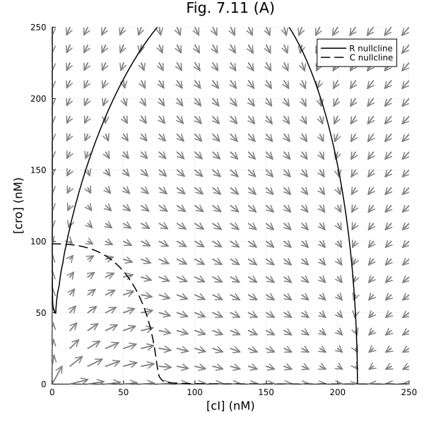
Fig 7.11 (B)
prob711b = remake(prob711, p=[delta_r => 0.2])
dx, dy = get_gradient(prob711b, r, c, xx, yy)
dxnorm, dynorm = normalize_gradient(dx[1:5:end, 1:5:end], dy[1:5:end, 1:5:end], 5*step(xrange), 5*step(yrange))
quiver(xx_sp, yy_sp, quiver=(dxnorm, dynorm); aspect_ratio=1, size=(600, 600), xlims=(0, 250), ylims=(0, 250), color=:gray)
contour!(xrange, yrange, dx, levels=[0], line=(:black, :solid), colorbar=false)
plot!([], [],  line=(:black, :solid), label="R nullcline")
contour!(xrange, yrange, dy, levels=[0],  line=(:black, :dash), colorbar=false)
plot!([], [], line=(:black, :dash), label="C nullcline")
plot!(xlabel="[cI] (nM)", ylabel="[cro] (nM)", title="Fig. 7.11 (B)", legend=:topright)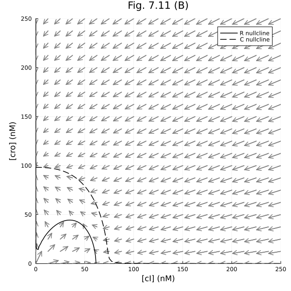
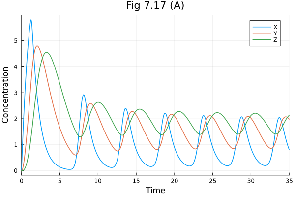
Fig 7.17
Goodwin oscillator model: Goodwin model (biology)
using OrdinaryDiffEq
using Catalyst
using Plots

@time "Build system" rn717 = @reaction_network begin
    (a / (k^n + Z^n), b), 0 <--> X
    (α * X, β), 0 <--> Y
    (γ * Y, δ), 0 <--> Z
end
Build system: 0.406405 seconds (1.51 M allocations: 74.702 MiB, 99.53% compilation time: 100% of which was recompilation)
Loading...
up717 = Dict(:a => 360.0, :k => 1.368, :b => 1.0, :α => 1.0, :β => 0.6, :γ => 1.0, :δ => 0.8, :n => 12.0, :X => 0.0, :Y => 0.0, :Z => 0.0)

tend = 35.0
@time "Build problem" prob717 = ODEProblem(rn717, up717, (0.0, tend))
@time "Solve problem" sol717 = solve(prob717, TRBDF2())
plot(sol717, idxs=[:X, :Y, :Z], labels=["X" "Y" "Z"], title="Fig 7.17 (A)", xlabel="Time", ylabel="Concentration")
Build problem: 1.248821 seconds (3.55 M allocations: 179.597 MiB, 2.16% gc time, 98.38% compilation time: 10% of which was recompilation)
Solve problem: 2.348799 seconds (5.39 M allocations: 287.063 MiB, 1.01% gc time, 99.71% compilation time)
plot(sol717, idxs=(:X, :Y, :Z), labels=false, title="Fig 7.17 (B)", size=(600, 600), xlabel="X", ylabel="Y", zlabel="Z")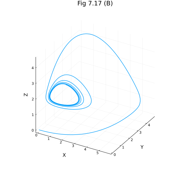
Fig 7.19
Circadian rhythm model
using OrdinaryDiffEq
using Catalyst
using Plots
Plots.gr(linewidth=1.5)

@time "Build system" rn719 = @reaction_network begin
    hillr(PN, vs, ki, n), 0 --> M
    mm(M, vm, km1), M => 0
    ks * M, 0 --> P0
    mm(P0, v1, k1), P0 => P1
    mm(P1, v2, k2), P1 => P0
    mm(P1, v3, k3), P1 => P2
    mm(P2, v4, k4), P2 => P1
    k1, P2 --> PN
    k2, PN --> P2
    mm(P2, vd, kd), P2 => 0
end
Build system: 0.227697 seconds (640.32 k allocations: 31.344 MiB, 99.40% compilation time)
Loading...
up719 = Dict(
    :vs => 0.76, :vm => 0.65, :vd => 0.95, :ks => 0.38, # :kt1 => 1.9, # :kt2 => 1.3,
    :v1 => 3.2, :v2 => 1.58, :v3 => 5.0, :v4 => 2.5,
    :k1 => 1.0, :k2 => 1.0, :k3 => 2.0, :k4 => 2.0, :ki => 1.0, :km1 => 0.5, :kd => 0.2, :n => 4,
    :M => 1.0, :P0 => 1.0, :P1 => 0.0, :P2 => 0.0, :PN => 0.0
)

tspan = (-50.0, 200.0)
@time "Build problem" prob719 = ODEProblem(rn719, up719, tspan)
@time "Solve problem" sol719 = solve(prob719, TRBDF2())
@unpack M, P0, P1, P2, PN = rn719
totalP = P0 + P1 + P2 + PN
plot(sol719, idxs=[M, PN, totalP], labels=["M" "Nuclear PER" "Total PER"], xlabel="Time", ylabel="Concentration", title="Fig 7.19 (A)")
Build problem: 1.336549 seconds (3.55 M allocations: 177.529 MiB, 2.07% gc time, 98.20% compilation time: <1% of which was recompilation)
Solve problem: 0.720670 seconds (1.61 M allocations: 81.186 MiB, 98.85% compilation time)
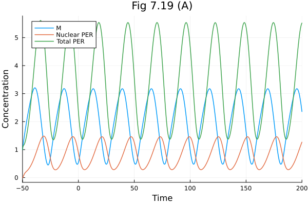
Fig 7.21
Repressilator model.
using OrdinaryDiffEq
using Catalyst
using Plots
Plots.gr(linewidth=1.5)

@time "Build system" rn721 = @reaction_network begin
    (α0 + hillr(C, α, 1, n), 1), 0 <--> mA
    (α0 + hillr(A, α, 1, n), 1), 0 <--> mB
    (α0 + hillr(B, α, 1, n), 1), 0 <--> mC
    (β * mA, β), 0 <--> A
    (β * mB, β), 0 <--> B
    (β * mC, β), 0 <--> C
end
Build system: 0.108578 seconds (238.20 k allocations: 11.987 MiB, 98.70% compilation time)
Loading...
up721 = Dict(
    :α => 298.2, :α0 => 0.03, :n => 2.0, :β => 0.2,
    :mA => 0.2, :mB => 0.3, :mC => 0.4,
    :A => 0.1, :B => 0.1, :C => 0.5
)

tend = 300.0
@time "Build problem" prob721 = ODEProblem(rn721, up721, (0.0, tend))
@time "Solve problem" sol721 = solve(prob721, TRBDF2())

plot(sol721, idxs=[:A, :B, :C], xlabel="Time", ylabel="Concentration", title="Fig 7.21", legend=:left)
Build problem: 0.737098 seconds (1.35 M allocations: 74.173 MiB, 95.63% compilation time: <1% of which was recompilation)
Solve problem: 0.684726 seconds (1.52 M allocations: 77.256 MiB, 98.81% compilation time)
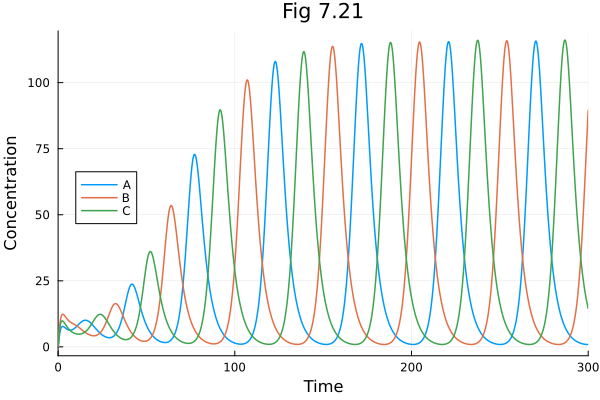
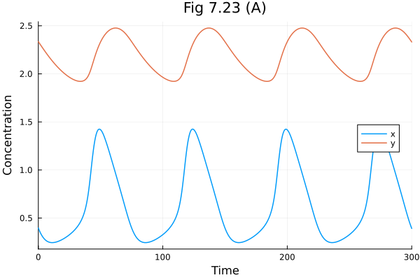
Fig 7.23
Hasty synthetic oscillator model
v0_723(x, y, alpha, sigma) = (1 + x^2 + alpha * sigma * x^4) / ((1 + x^2 + sigma * x^4) * (1 + y^4))
@time "Build system" rn723 = @reaction_network begin
    v0_723(x, y, alpha, sigma), 0 --> x
    ay * v0_723(x, y, alpha, sigma), 0 --> y
    gammax, x --> 0
    gammay, y --> 0
end
Build system: 0.357765 seconds (519.05 k allocations: 26.095 MiB, 7.30% gc time, 99.66% compilation time)
Loading...
up723 = Dict(
    :alpha => 11.0, :sigma => 2.0, :gammax => 0.2, :gammay => 0.012, :ay => 0.2,
    :x => 0.3963, :y => 2.3346,
)
tend = 300.0
@time "Build problem" prob723 = ODEProblem(rn723, up723, (0.0, tend))
@time "Solve problem" sol723 = solve(prob723, TRBDF2())
plot(sol723, idxs=[:x, :y], xlabel="Time", ylabel="Concentration", title="Fig 7.23 (A)", legend=:right)
Build problem: 0.690591 seconds (1.31 M allocations: 72.263 MiB, 97.36% compilation time)
Solve problem: 0.726866 seconds (1.66 M allocations: 84.537 MiB, 99.22% compilation time)
Vector field
xrange = range(0, 1.5, 51)
yrange = range(0, 3, 51)
@unpack x, y = rn723

xx, yy = meshgrid(xrange, yrange)
dx, dy = get_gradient(prob723, x, y, xx, yy)
contour(xrange, yrange, dx, levels=[0], line=(:black, :solid), colorbar=false)
plot!([], [], line=(:black, :solid), label="x nullcline")
contour!(xrange, yrange, dy, levels=[0], line=(:black, :dash), colorbar=false)
plot!([], [], line=(:black, :dash), label="y nullcline")
plot!(sol723, idxs=(x, y), label="Trajectory")
plot!(xlabel="x", ylabel="y", title="Fig 7.23 (B)", legend=:bottomright, size=(600, 600))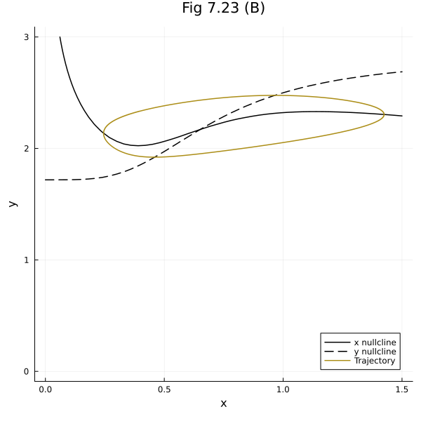
Fig 7.25
model of quorum sensing mechanism of Vibrio fischeri
using OrdinaryDiffEq
using SteadyStateDiffEq
using Catalyst
using ModelingToolkit
using ModelingToolkit: t_nounits as t, D_nounits as D
using Plots
Model with/without feedback
function build_sys725(; feedback=true, simplify=true, name=:model725)
    hil(x, k) = x / (k + x)
    hil(x, k, n) = hil(x^n, k^n)
    @parameters k0 = 0.0008 k1 = 0.5 k2 = 0.02 n = 0.6 a = 10 b = 0.07 a0 = 0.05 KM = 0.01 RT = 0.5 diff = 1000 popsize = 1000
    @variables A(t) = 0 I(t) = 0 Rstar(t) = 0 Aout(t) = 0 R0(t)
    R0 = RT - 2Rstar
    v0 = feedback ? k0 * I : k0 * 15.0
    v1 = k1 * A^2 * R0^2
    v2 = k2 * Rstar
    va = n * (A - Aout)
    eqs = [
        R0 ~ RT - 2Rstar,
        D(A) ~ v0 - 2v1 + 2v2 - va,
        D(I) ~ a0 + a * hil(Rstar, KM) - b * I,
        D(Rstar) ~ v1 - v2,
        D(Aout) ~ popsize * va - diff * Aout
    ]
    sys = ODESystem(eqs, t; name)
    return simplify ? mtkcompile(sys) : sys
end
build_sys725 (generic function with 1 method)@time "Build system" sys725 = build_sys725()
@time "Build system" sys725_no_feedback = build_sys725(feedback=false)
@time "Build problem" prob725 = SteadyStateProblem(sys725, [])
@time "Build problem" prob725_no_feedback = SteadyStateProblem(sys725_no_feedback, [])Build system: 1.206222 seconds (1.84 M allocations: 89.013 MiB, 2.36% gc time, 99.67% compilation time)
Build system: 0.184224 seconds (189.22 k allocations: 9.108 MiB, 97.65% compilation time)
Build problem: 3.616007 seconds (7.23 M allocations: 378.782 MiB, 0.70% gc time, 99.37% compilation time: 73% of which was recompilation)
Build problem: 0.359688 seconds (755.85 k allocations: 40.445 MiB, 97.33% compilation time)
SteadyStateProblem with uType Vector{Float64}. In-place: true
u0: 4-element Vector{Float64}:
 0.0
 0.0
 0.0
 0.0
npops = 1:50:5001
trajectories = length(npops)
alg = DynamicSS(KenCarp47())
@unpack popsize, I = sys725
prob_func = (prob, i, repeat) -> remake(prob, p=[popsize => npops[i]])
eprob = EnsembleProblem(prob725; prob_func)
eprob_nofeed = EnsembleProblem(prob725_no_feedback; prob_func)
@time sim = solve(eprob, alg; trajectories);
@time sim_no_feed = solve(eprob_nofeed, alg; trajectories); 5.907751 seconds (15.12 M allocations: 867.751 MiB, 6.88% gc time, 41730 lock conflicts, 288.33% compilation time)
6.293523 seconds (13.16 M allocations: 770.044 MiB, 1.78% gc time, 44729 lock conflicts, 203.78% compilation time)
luxI = map(s -> s[I], sim)
luxI_nofeed = map(s -> s[I], sim_no_feed)
plot(npops, [luxI, luxI_nofeed], xscale=:log10, xlabel="Population size", ylabel="LuxI concentration (μM)", title="Fig. 7.25", label=["With feedback" "Without feedback"], legend=:topleft)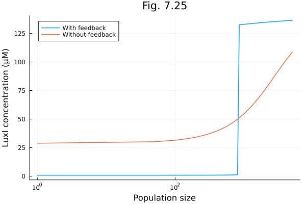
Fig 7.28
model of synthetic pulse generating system
using OrdinaryDiffEq
using Catalyst
using Plots

function vg728(R, C, KR, KC, aG)
    fR = R / KR
    fC = C / KC
    return aG * (fR / (1 + fR + fC^2 + fR * fC^2))
end

@time "Build system" rn728 = @reaction_network begin
    vg728(R, C, KR, KC, aG), 0 --> G
    bG, G --> 0
    mm(R, aC, KR), 0 --> C
    bC, C --> 0
    k1 * (RT - 2R)^2 * A^2, 0 --> R
    k2, R --> 0
end
Build system: 0.046577 seconds (197.00 k allocations: 9.806 MiB, 96.92% compilation time)
Loading...
up728 = Dict(
    :aG => 80.0, # muM/min
    :bG => 0.07, # /min
    :KC => 0.008, # muM
    :aC => 0.5, # muM/min
    :bC => 0.3, # /min
    :k1 => 0.5, # /muM^3 /min
    :k2 => 0.02, # /min
    :KR => 0.02, # muM
    :RT => 0.5, # muM
    :A => 10.0, # muM
    :G => 0.0,
    :C => 0.0,
    :R => 0.0,
)

tend = 50.0
@time "Build problem" prob728 = ODEProblem(rn728, up728, (0.0, tend))
@time "Solve problem" sol728 = solve(prob728, TRBDF2())

plot(sol728, idxs=[:G, :C, :R], xlabel="Time (min)", ylabel="Concentration (μM)", title="Fig 7.28", label=["GFP" "cI" "LuxR:AHL complex"])
Build problem: 0.703494 seconds (1.32 M allocations: 72.425 MiB, 97.12% compilation time)
Solve problem: 0.684304 seconds (1.57 M allocations: 80.182 MiB, 99.14% compilation time)
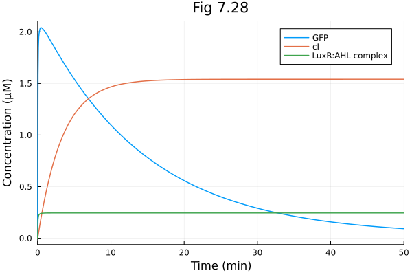
Fig. 7.30
model of synthetic band detector system
using OrdinaryDiffEq
using SteadyStateDiffEq
using Catalyst
using Plots
Plots.gr(linewidth=1.5)

@time "Build system" rn730 = @reaction_network begin
    hillr(L, aG, KL, 2), 0 --> G
    bG, G --> 0
    hillr(C, aL1, KC, 2), 0 --> L
    mm(R, aL2, KR), 0 --> L
    bL, L --> 0
    mm(R, aC, KR), 0 --> C
    bC, C --> 0
    k1 * (RT - 2R)^2 * A^2, 0 --> R
    k2, R --> 0
end
Build system: 0.029285 seconds (182.07 k allocations: 9.000 MiB, 95.75% compilation time)
Loading...
up730 = Dict(
    :aG => 2.0, # muM/min
    :bG => 0.07, # /min
    :KL => 0.8, # muM
    :aL1 => 1, # muM/min
    :aL2 => 1, # muM/min
    :KC => 0.008, # muM
    :bL => 0.02, # /min
    :aC => 1, # muM/min
    :bC => 0.07, # /min
    :k1 => 0.5, # /muM^3 /min
    :k2 => 0.02, # /min
    :KR => 0.01, # muM
    :RT => 0.5, # muM
    :A => 0.1,
    :G => 0.0,
    :L => 0.0,
    :C => 0.0,
    :R => 0.0,
)

(sols, as) = let N = 1:100
    as = [exp10(-4 + 4 * (i - 1) / length(N)) for i in N]
    @time "Build problem" prob = SteadyStateProblem(rn730, up730)
    prob_func = (prob, i, repeat) -> remake(prob, p=[:A => as[i]])
    eprob = EnsembleProblem(prob; prob_func)
    @time "Solve problem" sols = solve(eprob, DynamicSS(TRBDF2()); trajectories=length(N))
    (sols, as)
end;
Build problem: 1.174864 seconds (3.52 M allocations: 179.195 MiB, 6.89% gc time, 98.36% compilation time)
Solve problem: 5.688155 seconds (13.57 M allocations: 794.961 MiB, 6.60% gc time, 42105 lock conflicts, 234.59% compilation time)
luxI = map(s -> s[:L], sols)
CI = map(s -> s[:C], sols)
GFP = map(s -> s[:G], sols)
plot(as, [luxI, CI, GFP], xscale=:log10, xlabel="AHL concentration (μM)", ylabel="Concentration (μM)", title="Fig. 7.30", label=["LuxI" "cI" "GFP"])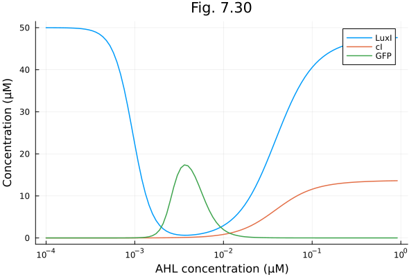
Fig. 7.31
Hasty synthetic oscillator model
using OrdinaryDiffEq
using Catalyst
using Plots
Plots.gr(linewidth=1.5)

v0_731(x, y, alpha, sigma) = (1 + x^2 + alpha * sigma * x^4) / ((1 + x^2 + sigma * x^4) * (1 + y^4))
@time "Build system" rn731 = @reaction_network begin
    v0_731(x1, y1, alpha, sigma), 0 --> x1
    ay * v0_731(x1, y1, alpha, sigma), 0 --> y1
    v0_731(x2, y2, alpha, sigma), 0 --> x2
    ay * v0_731(x2, y2, alpha, sigma), 0 --> y2
    gammax, x1 --> 0
    gammay, y1 --> 0
    gammax, x2 --> 0
    gammay, y2 --> 0
    (D, D), x1 <--> x2
    (D, D), y1 <--> y2
end
Build system: 0.009964 seconds (9.01 k allocations: 373.250 KiB, 84.60% compilation time)
Loading...
up731 = Dict(
    :alpha => 11.0,
    :sigma => 2.0,
    :gammax => 0.2,
    :gammay => 0.012,
    :ay => 0.2,
    :D => 0.015,
    :x1 => 0.3963,
    :y1 => 2.3346,
    :x2 => 0.5578,
    :y2 => 1.9317,
)

tend = 500.0
@time "Build problem" prob731 = ODEProblem(rn731, up731, (0.0, tend))
@time "Solve problem" sol731 = solve(prob731, TRBDF2())
plot(sol731, xlabel="Time (a.u.)", ylabel="Concentration (a.u.)", title="Fig. 7.31", legend=:left)
Build problem: 0.690052 seconds (1.39 M allocations: 75.917 MiB, 95.44% compilation time)
Solve problem: 0.745922 seconds (1.90 M allocations: 96.095 MiB, 99.07% compilation time)
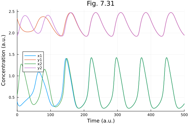
Fig. 7.38
stochastic implementation (Gillespie SSA) of a collection of spontaneously decaying molecules.
using JumpProcesses
using Catalyst
using Plots

@time "Build system" rn738 = @reaction_network begin
    d, A --> 0
end
Build system: 0.048884 seconds (53.14 k allocations: 2.559 MiB, 98.29% compilation time)
Loading...
tend = 5.0
ps738 = Dict(:d => 1.0)
@time "Build problem" jprob1000 = JumpProblem(rn738, [:A => 1000], (0.0, tend), ps738)
jprob100 = remake(jprob1000, u0=[:A => 100])
jprob10 = remake(jprob1000, u0=[:A => 10])

@time "Solve problem" sol1000 = solve(jprob1000)
@time "Solve problem" sol100 = solve(jprob100)
@time "Solve problem" sol10 = solve(jprob10)
Build problem: 6.286975 seconds (16.55 M allocations: 835.631 MiB, 2.63% gc time, 99.93% compilation time)
Solve problem: 0.312252 seconds (804.18 k allocations: 39.743 MiB, 99.95% compilation time)
Solve problem: 0.000050 seconds (232 allocations: 14.500 KiB)
Solve problem: 0.000034 seconds (50 allocations: 4.109 KiB)
retcode: Success
Interpolation: Piecewise constant interpolation
t: 12-element Vector{Float64}:
 0.0
 0.0017264199760988635
 0.013817454155656253
 0.2552362835191831
 0.3834592804199417
 1.1369446413997242
 1.5651441573727412
 1.8025289116278
 2.1263495039657423
 3.0634465761144822
 3.2290752489567085
 5.0
u: 12-element Vector{Vector{Int64}}:
 [10]
 [9]
 [8]
 [7]
 [6]
 [5]
 [4]
 [3]
 [2]
 [1]
 [0]
 [0]
plot(sol1000, xlabel="Time", ylabel="# of molecules", title="Fig. 7.38 (A)", label="1000 molecules")
plot!(t -> 1000 * exp(-t), linestyle=:dash, label="ODE solution")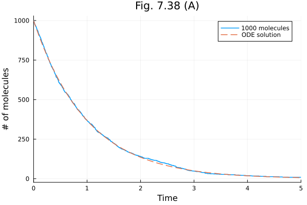
plot(sol100, xlabel="Time", ylabel="# of molecules", title="Fig. 7.38 (B)", label="100 molecules")
plot!(t -> 100 * exp(-t), linestyle=:dash, label="ODE solution")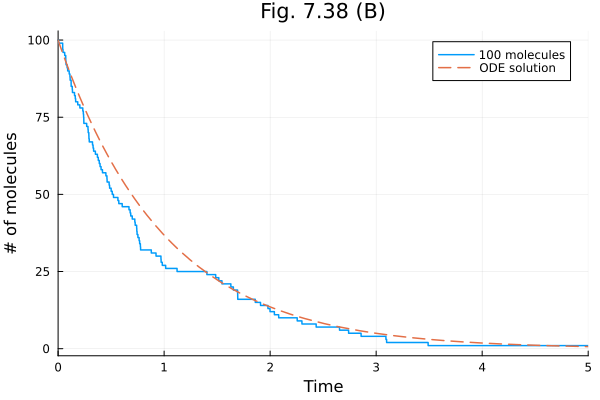
plot(sol10, xlabel="Time", ylabel="# of molecules", title="Fig. 7.38 (C)", label="10 molecules")
plot!(t -> 10 * exp(-t), linestyle=:dash, label="ODE solution")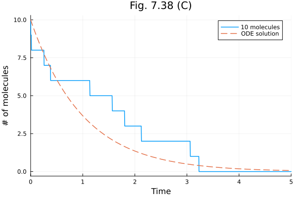
This notebook was generated using Literate.jl.