Fig 4.7, 4.8

Symmetric (bistable) biological networks.

using OrdinaryDiffEq
using ComponentArrays: ComponentArray
using SimpleUnPack
using CairoMakie

Model

function model407(u, p, t)
    @unpack A, B = u
    @unpack k1, k2, k3, k4, n1, n2 = p
    dA = k1 / (1 + B^n1) - k3 * A
    dB = k2 / (1 + A^n2) - k4 * B
    return (; dA, dB)
end
function model407!(D, u, p, t)
    @unpack dA, dB = model407(u, p, t)
    D.A = dA
    D.B = dB
    nothing
end

model407! (generic function with 1 method)

Fig 4.7 A¶

Asymmetric parameter set

ps407 = ComponentArray(k1 = 20.0,k2 = 20.0,k3 = 5.0,k4 = 5.0, n1 = 4.0, n2 = 1.0)
ics407 = ComponentArray( A = 3.0, B = 1.0)
tend = 4.0
prob407 = ODEProblem(model407!, ics407, (0.0, tend), ps407)

ODEProblem with uType ComponentArrays.ComponentVector{Float64, Vector{Float64}, Tuple{ComponentArrays.Axis{(A = 1, B = 2)}}} and tType Float64. In-place: true
Non-trivial mass matrix: false
timespan: (0.0, 4.0)
u0: ComponentVector{Float64}(A = 3.0, B = 1.0)

@time sol1 = solve(prob407, Tsit5())
@time sol2 = solve(remake(prob407, u0=ComponentArray(A=1.0, B=3.0)), Tsit5())
fig = Figure(size=(600, 600))
ax1 = Axis(fig[1, 1], xlabel="Time", ylabel="Concentration", title= "Fig 4.7A (1)")
lines!(ax1, 0..tend, t-> sol1(t).A, label="A")
lines!(ax1, 0..tend, t-> sol1(t).B, label="B")
axislegend(ax1, position=:rc)
ax2 = Axis(fig[2, 1], xlabel="Time", ylabel="Concentration", title= "Fig 4.7A (2)")
lines!(ax2, 0..tend, t-> sol2(t).A, label="A")
lines!(ax2, 0..tend, t-> sol2(t).B, label="B")
axislegend(ax2, position=:rc)
fig

  0.881326 seconds (4.75 M allocations: 316.269 MiB, 15.30% gc time, 100.00% compilation time)
  0.014085 seconds (103.75 k allocations: 7.336 MiB, 99.47% compilation time)

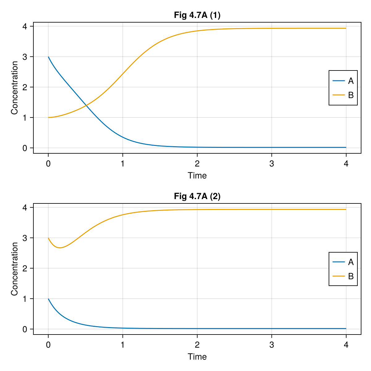
Fig 4.7 B¶

Vector field with nullclines

∂F47 = function (x, y)
    @unpack dA, dB = model407((; A=x, B=y), ps407, nothing)
    return Point2d(dA, dB)
end

fig = Figure(size=(600, 600))
ax = Axis(fig[1, 1],
    xlabel = "[A]",
    ylabel = "[B]",
    title = "Fig 4.7 B\nVector field with nullclines",
    aspect = 1,
)

# Nullclines
let xrange = 0:0.01:5, yrange = 0:0.01:5
    zA47 = [model407((; A=x, B=y), ps407, nothing).dA for x in xrange, y in yrange]
    zB47 = [model407((; A=x, B=y), ps407, nothing).dB for x in xrange, y in yrange]
    contour!(ax, xrange, yrange, zA47, levels=[0], color=:black, label="A nullcline", linewidth=2, linestyle=:solid)
    contour!(ax, xrange, yrange, zB47, levels=[0], color=:black, label="B nullcline", linewidth=2, linestyle=:dash)
end

# Vector field
streamplot!(ax, ∂F47, 0..5, 0..5)
limits!(ax, 0.0, 5.0, 0.0, 5.0)
axislegend(ax, position = :rc)
fig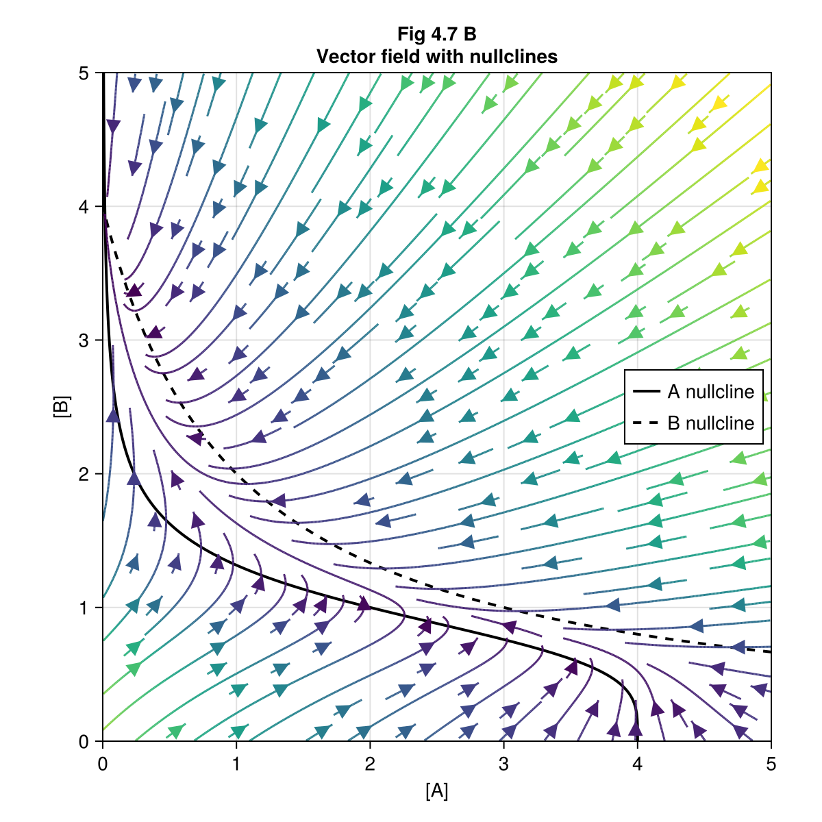

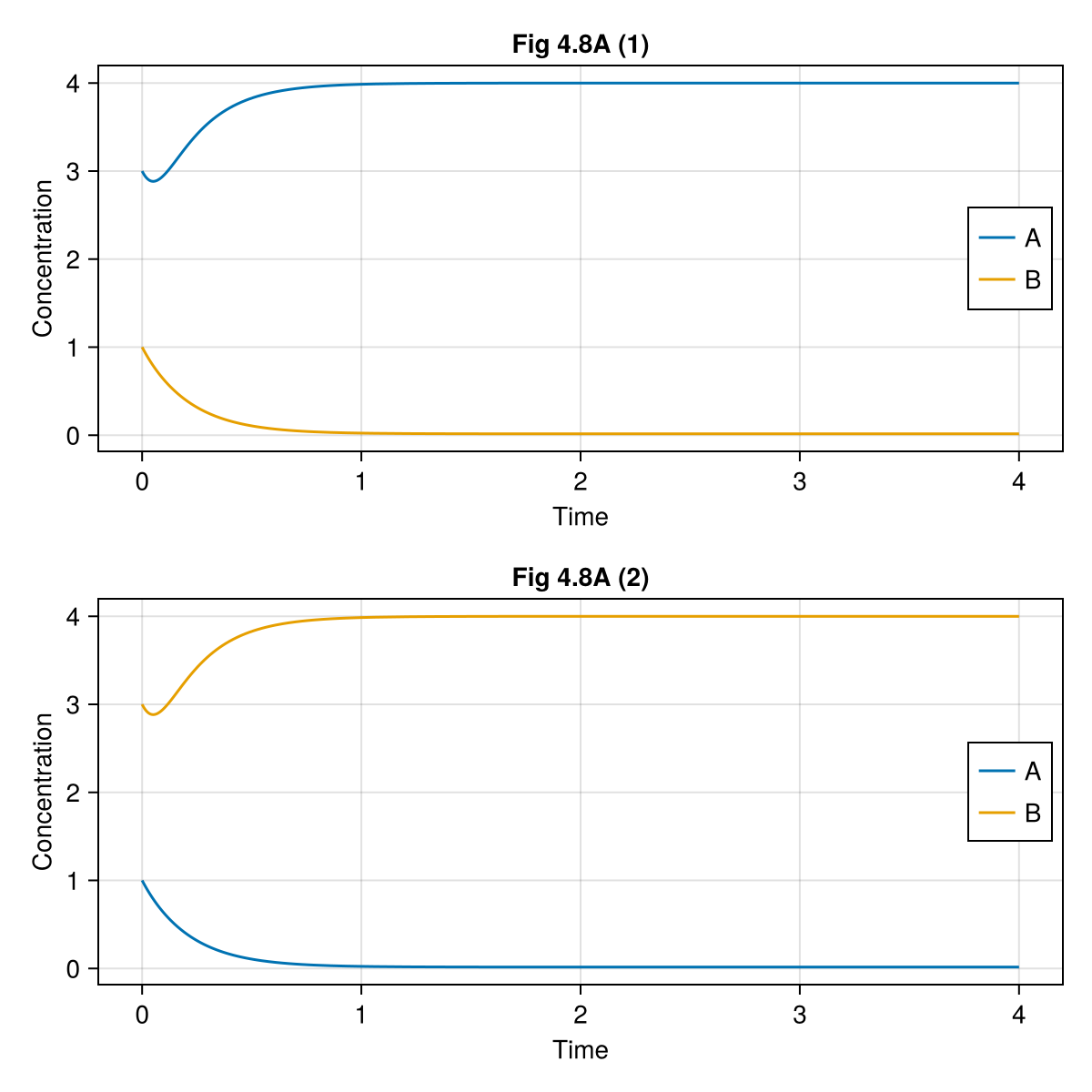
Fig 4.8¶

Symmetric parameter set

ps408 = ComponentArray(k1 = 20.0, k2 = 20.0, k3 = 5.0, k4 = 5.0, n1 = 4.0, n2 = 4.0)
ics408 = ComponentArray(A = 3.0, B = 1.0)
tend = 4.0
prob408 = ODEProblem(model407!, ics408, (0.0, tend), ps408)

@time sol1 = solve(prob408, Tsit5())
@time sol2 = solve(remake(prob408, u0=ComponentArray(A=1.0, B=3.0)), Tsit5())

fig = Figure(size=(600, 600))
ax1 = Axis(fig[1, 1], xlabel="Time", ylabel="Concentration", title= "Fig 4.8A (1)")
lines!(ax1, 0..tend, t-> sol1(t).A, label="A")
lines!(ax1, 0..tend, t-> sol1(t).B, label="B")
axislegend(ax1, position=:rc)
ax2 = Axis(fig[2, 1], xlabel="Time", ylabel="Concentration", title= "Fig 4.8A (2)")
lines!(ax2, 0..tend, t-> sol2(t).A, label="A")
lines!(ax2, 0..tend, t-> sol2(t).B, label="B")
axislegend(ax2, position=:rc)
fig

  0.000024 seconds (242 allocations: 19.727 KiB)
  0.000048 seconds (268 allocations: 21.070 KiB)

∂F48 = function (x, y)
    @unpack dA, dB = model407((; A=x, B=y), ps408, nothing)
    return Point2d(dA, dB)
end

#23 (generic function with 1 method)

fig = Figure(size=(600, 600))
ax = Axis(fig[1, 1],
    xlabel = "[A]",
    ylabel = "[B]",
    title = "Fig 4.8 B\nVector field with nullclines",
    aspect = 1,
)

let xs = 0.0:0.01:5.0, ys = 0.0:0.01:5.0
    zA48 = [model407((; A=x, B=y), ps408, nothing).dA for x in xs, y in ys]
    zB48 = [model407((; A=x, B=y), ps408, nothing).dB for x in xs, y in ys]
    contour!(ax, xs, ys, zA48, levels=[0], color=:black, label="A nullcline", linewidth=2, linestyle=:solid)
    contour!(ax, xs, ys, zB48, levels=[0], color=:black, label="B nullcline", linewidth=2, linestyle=:dash)
end
streamplot!(ax, ∂F48, 0..5, 0..5)
limits!(ax, 0.0, 5.0, 0.0, 5.0)
axislegend(ax, position = :rc)
fig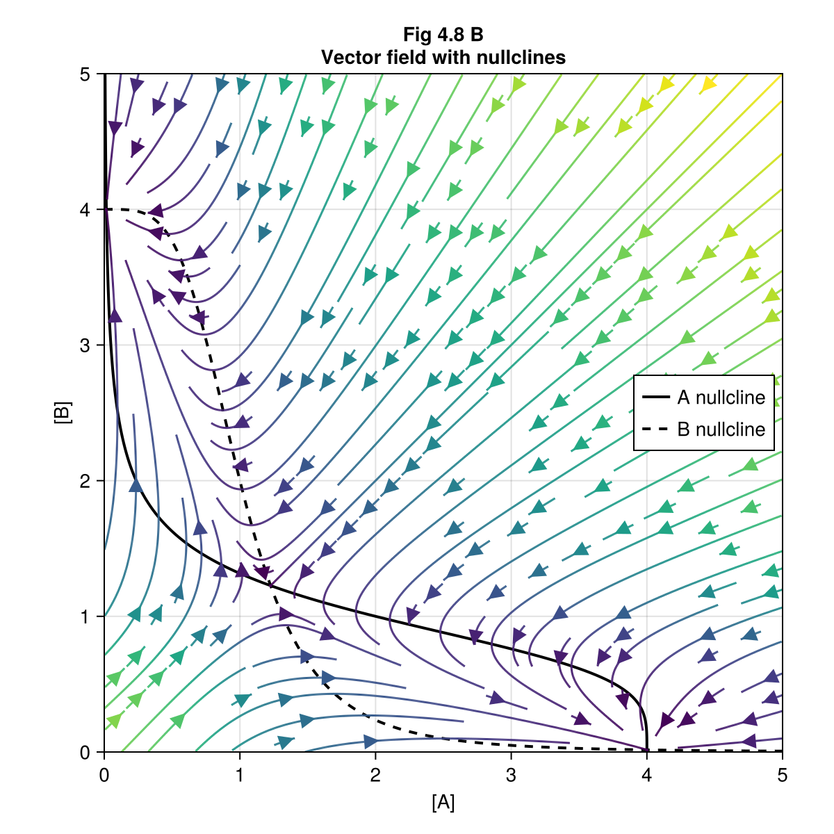

Fig 4.8 C¶

Around the unstable steady-state

fig = Figure(size=(600, 600))
ax = Axis(fig[1, 1],
    xlabel = "[A]",
    ylabel = "[B]",
    title = "Fig 4.8 C\nClose-up of vector field with nullclines",
    aspect = 1,
)

let xs = 1.0:0.005:1.5, ys = 1.0:0.005:1.5
    zA48 = [model407((; A=x, B=y), ps408, nothing).dA for x in xs, y in ys]
    zB48 = [model407((; A=x, B=y), ps408, nothing).dB for x in xs, y in ys]
    contour!(ax, xs, ys, zA48, levels=[0], color=:black, label="A nullcline", linewidth=2, linestyle=:solid)
    contour!(ax, xs, ys, zB48, levels=[0], color=:black, label="B nullcline", linewidth=2, linestyle=:dash)
end
streamplot!(ax, ∂F48, 1.0..1.5, 1.0..1.5)
limits!(ax, 1.0, 1.5, 1.0, 1.5)
axislegend(ax, position = :rc)
fig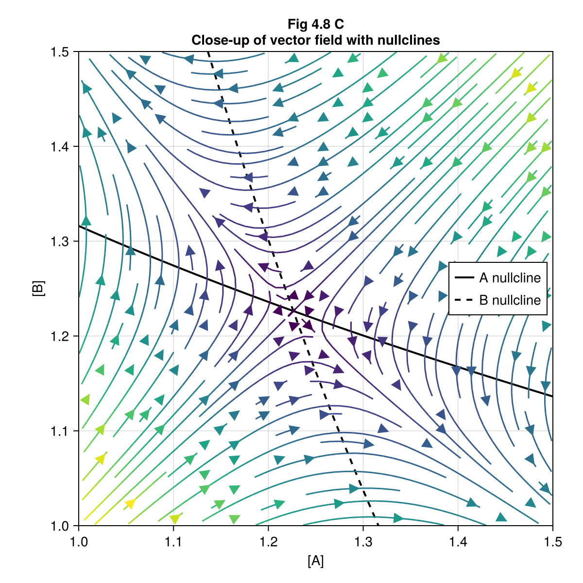

Another way to draw nullclines is to find the analytical solutions for dA (or dB) is zero. And then sketch the nullclines in a parameteric plot.

nca47(b, p) = p.k1 / p.k3 / (1 + b^p.n1)
ncb47(a, p) = p.k2 / p.k4 / (1 + a^p.n2)

fig = Figure(size = (800, 800))
for (i, k1) in enumerate((8.0, 16.0, 20.0, 35.0))
    ps = (k1=k1, k2=20., k3=5., k4=5., n1=4., n2=4.)
    ax = Axis(fig[div(i-1,2)+1, mod(i-1,2)+1],
        xlabel = "[A]",
        ylabel = "[B]",
        title = "K1 = $k1",
        aspect = 1,
    )
    ts = 0:0.01:7
    aa = nca47.(ts, Ref(ps))
    bb = ncb47.(ts, Ref(ps))
    lines!(ax, aa, ts, color=:red, label="Nullcline A")
    lines!(ax, ts, bb, color=:blue, label="Nullcline B")
    limits!(ax, 0, 7, 0, 7)
    axislegend(ax, position = :rc)
end
fig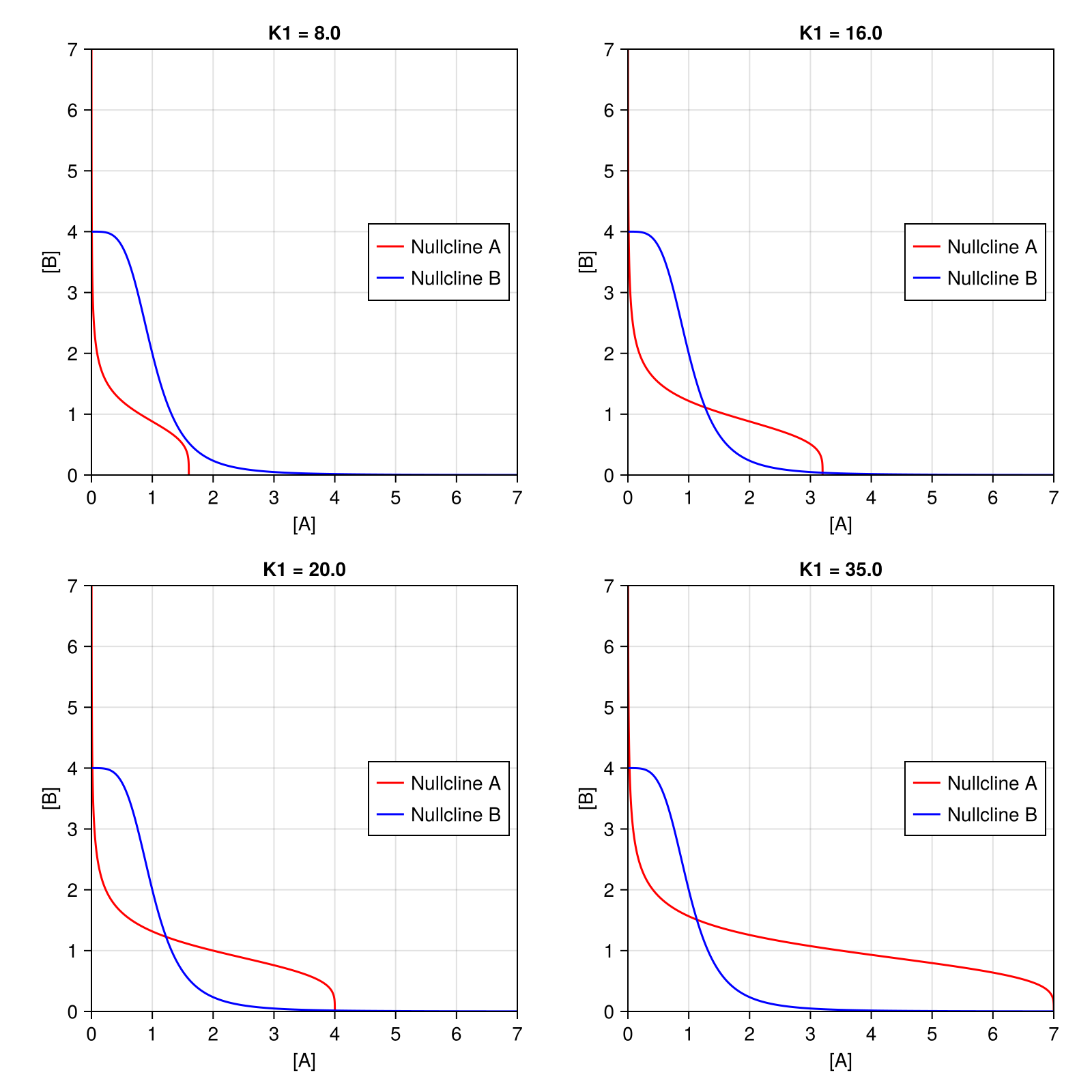

This notebook was generated using Literate.jl.