Fig 4.2, 4.3, 4.4, 4.5

Steady states and phase plots in an asymmetric network.

using OrdinaryDiffEq
using ComponentArrays: ComponentArray
using SimpleUnPack
using CairoMakie

The model for figure 4.1, 4.2, and 4.3.

function model401(u, p, t)
    @unpack A, B = u
    @unpack k1, k2, k3, k4, k5, n = p
    dA = k1 / (1 + B^n) - (k3 + k5) * A
    dB = k2 + k5 * A - k4 * B
    return (; dA, dB)
end
function model401!(D, u, p, t)
    @unpack dA, dB = model401(u, p, t)
    D.A = dA
    D.B = dB
    return nothing
end

model401! (generic function with 1 method)

Fig 4.2 A¶

tend = 1.5
ps402a = ComponentArray(k1=20.0, k2=5.0, k3=5.0, k4=5.0, k5=2.0, n=4.0)
ics402a = ComponentArray(A=0.0, B=0.0)
prob401 = ODEProblem(model401!, ics402a, tend, ps402a)

u0s = [
    ComponentArray(
        A=a,
        B=b
    ) for (a, b) in [
        [0.0, 0.0],
        [0.5, 0.6],
        [0.17, 1.1],
        [0.25, 1.9],
        [1.85, 1.7]]
]

5-element Vector{ComponentArrays.ComponentVector{Float64, Vector{Float64}, Tuple{ComponentArrays.Axis{(A = 1, B = 2)}}}}:
 ComponentVector{Float64}(A = 0.0, B = 0.0)
 ComponentVector{Float64}(A = 0.5, B = 0.6)
 ComponentVector{Float64}(A = 0.17, B = 1.1)
 ComponentVector{Float64}(A = 0.25, B = 1.9)
 ComponentVector{Float64}(A = 1.85, B = 1.7)

@time sols = map(u0s) do u0
    solve(remake(prob401, u0=u0), Tsit5())
end

  0.926720 seconds (5.07 M allocations: 338.592 MiB, 8.46% gc time, 99.97% compilation time)

fig = Figure()
ax = Axis(fig[1, 1],
    xlabel="Time",
    ylabel="Concentration",
    title="Fig. 4.2 A\nTime series"
)
lines!(ax, 0 .. tend, t -> sols[1](t).A, label="A")
lines!(ax, 0 .. tend, t -> sols[1](t).B, label="B")
axislegend(ax, position=:rt)
fig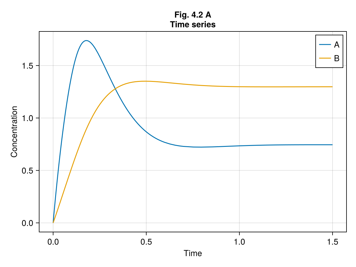

Fig. 4.2 B (Phase plot)¶

fig = Figure(size=(600, 600))
ax = Axis(fig[1, 1],
    xlabel="[A]",
    ylabel="[B]",
    title="Fig. 4.2 B\nPhase plot",
    aspect=1,
)
let ts = 0:0.01:tend
    aa = [sols[1](t).A for t in ts]
    bb = [sols[1](t).B for t in ts]
    lines!(ax, aa, bb)
end
limits!(ax, 0.0, 2.0, 0.0, 2.0)
fig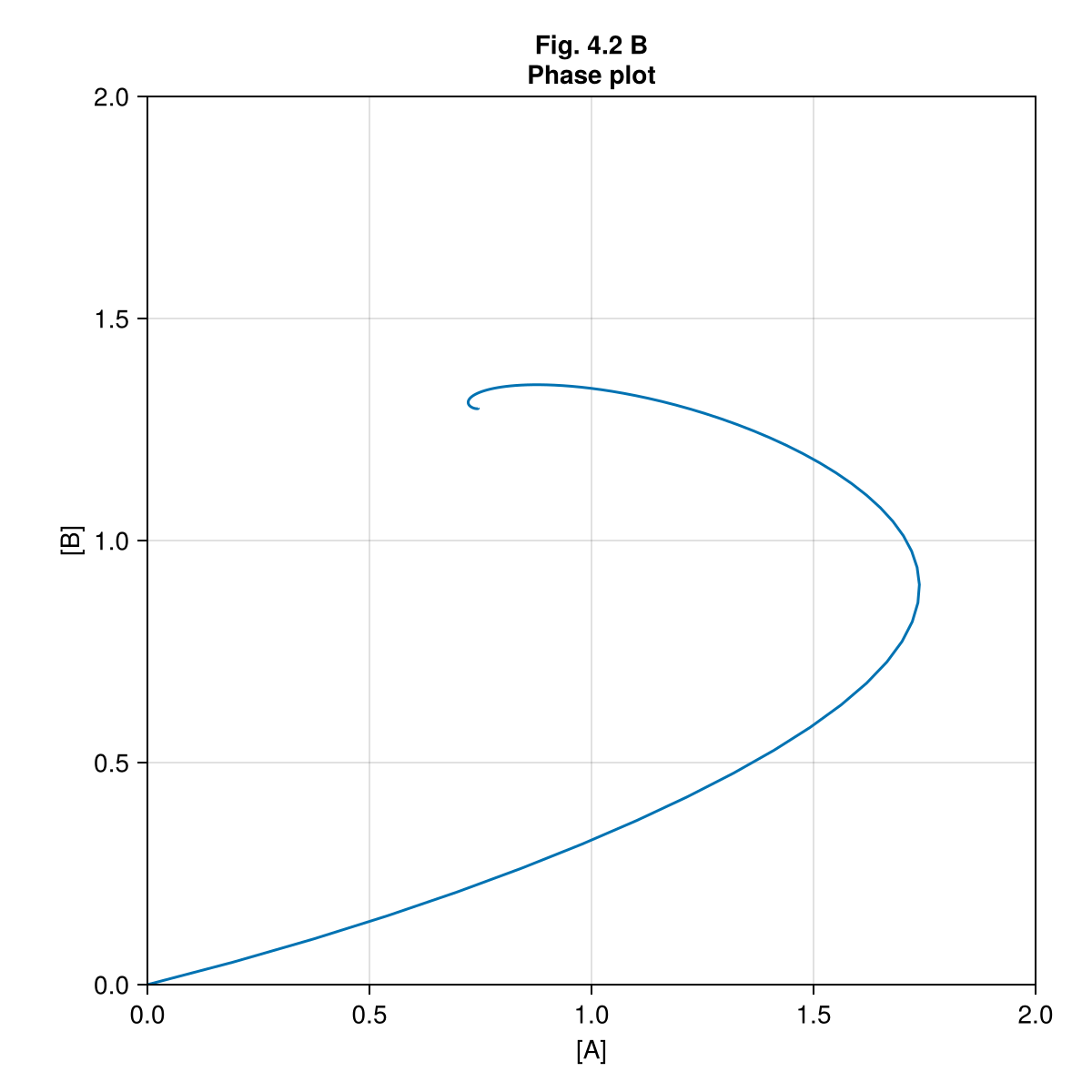

Fig. 4.3 A (Multiple time series)¶

fig = Figure()
ax = Axis(fig[1, 1],
    xlabel="Time",
    ylabel="Concentration",
    title="Fig. 4.3A\nMultiple time series"
)
for sol in sols
    lines!(ax, 0 .. tend, t -> sol(t).A, alpha=0.7)
    lines!(ax, 0 .. tend, t -> sol(t).B, alpha=0.7)
end
fig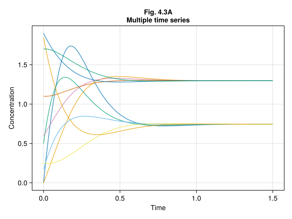

Fig. 4.3 B (Phase plot)¶

fig = Figure(size=(600, 600))
ax = Axis(fig[1, 1],
    xlabel="[A]",
    ylabel="[B]",
    title="Fig. 4.3 B\nPhase plot",
    aspect=1,
)

for sol in sols
    ts = 0:0.01:tend
    aa = [sol(t).A for t in ts]
    bb = [sol(t).B for t in ts]
    lines!(ax, aa, bb)
end
limits!(ax, 0.0, 2.0, 0.0, 2.0)
fig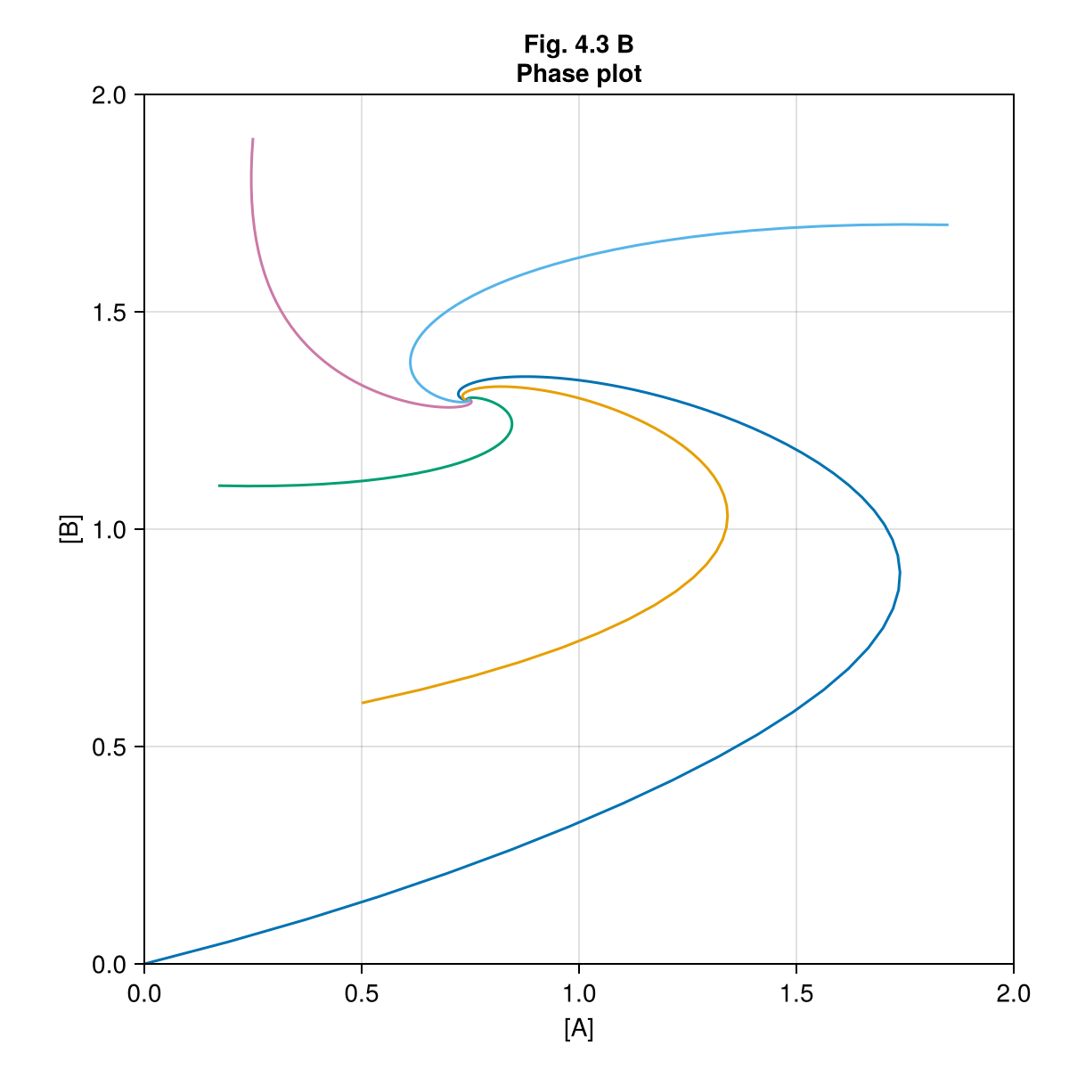

Let’s sketch vector fields in phase plots

∂F44 = function (x, y)
    @unpack dA, dB = model401((; A=x, B=y), ps402a, nothing)
    Point2d(dA, dB)
end

fig = Figure(size=(600, 600))
ax = Axis(fig[1, 1],
    xlabel="[A]",
    ylabel="[B]",
    title="Fig. 4.4 A\nPhase plot with vector field",
    aspect=1,
)

streamplot!(ax, ∂F44, 0 .. 2, 0 .. 2)
for sol in sols
    ts = 0:0.01:tend
    aa = [sol(t).A for t in ts]
    bb = [sol(t).B for t in ts]
    lines!(ax, aa, bb, color=:black)
end
limits!(ax, 0.0, 2.0, 0.0, 2.0)
fig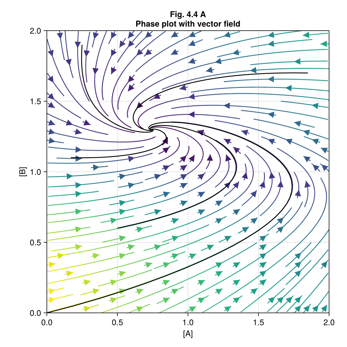

Figure 4.5A¶

fig = Figure(size=(600, 600))
ax = Axis(fig[1, 1],
    xlabel="[A]",
    ylabel="[B]",
    title="Fig. 4.5 A\nPhase plot with nullclines",
    aspect=1,
)

# Phase plots
for sol in sols
    ts = 0:0.01:tend
    aa = [sol(t).A for t in ts]
    bb = [sol(t).B for t in ts]
    lines!(ax, aa, bb)
end

# nullclines
xs = 0:0.01:2
ys = 0:0.01:2
zA44 = [model401((; A=x, B=y), ps402a, nothing).dA for x in xs, y in ys]
zB44 = [model401((; A=x, B=y), ps402a, nothing).dB for x in xs, y in ys]
contour!(ax, xs, ys, zA44, levels=[0], color=:black, linestyle=:solid, linewidth=2, label="A nullcline")
contour!(ax, xs, ys, zB44, levels=[0], color=:black, linestyle=:dash, linewidth=2, label="B nullcline")
limits!(ax, 0.0, 2.0, 0.0, 2.0)
axislegend(ax, position=:rb)
fig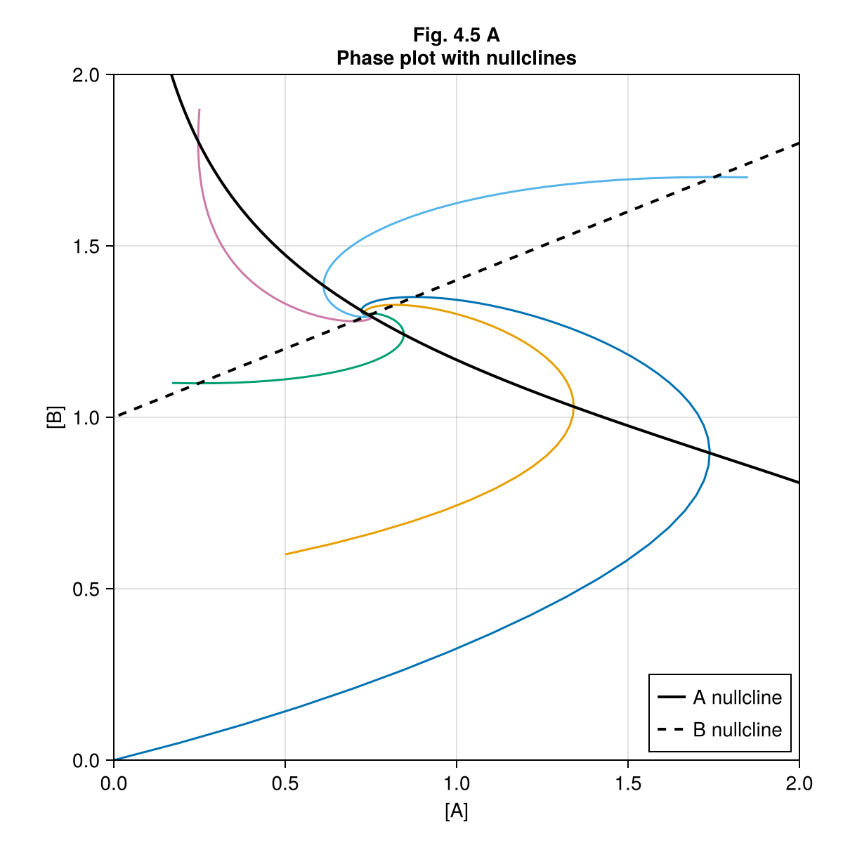

Figure 4.5 B¶

Vector field with nullclines

fig = Figure(size=(600, 600))
ax = Axis(fig[1, 1],
    xlabel="[A]",
    ylabel="[B]",
    title="Fig. 4.5 B\nVector field with nullclines",
    aspect=1,
)
contour!(ax, xs, ys, zA44, levels=[0], color=:black, linestyle=:solid, linewidth=2, label="A nullcline")
contour!(ax, xs, ys, zB44, levels=[0], color=:black, linestyle=:dash, linewidth=2, label="B nullcline")
streamplot!(ax, ∂F44, 0 .. 2, 0 .. 2)
limits!(ax, 0.0, 2.0, 0.0, 2.0)
fig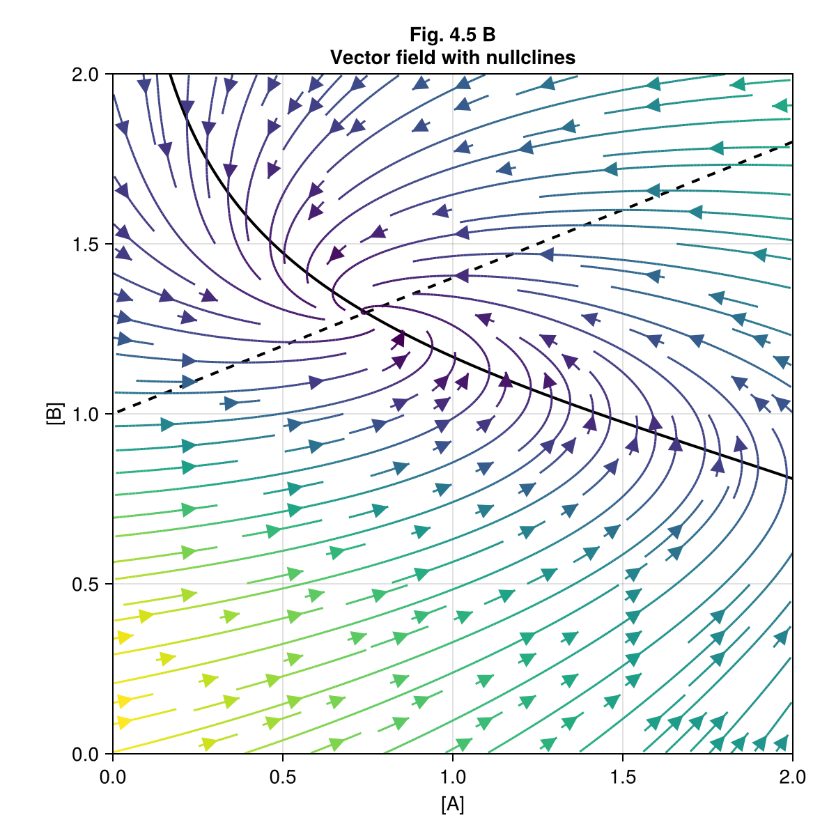

This notebook was generated using Literate.jl.