Solving differential equations in Julia

Standard procedures

Define a model function representing the right-hand-side (RHS) of the system.
- Out-of-place form: f(u, p, t) where u is the state variable(s), p is the parameter(s), and t is the independent variable (usually time). The output is the right hand side (RHS) of the differential equation system.
- In-place form: f!(du, u, p, t), where the output is saved to du. The rest is the same as the out of place form. The in-place form has potential performance benefits since it allocates less than the out-of-place (f(u, p, t)) counterpart.
- Using ModelingToolkit.jl : define equations and build an ODE system.
Initial conditions (u0) for the state variable(s).
(Optional) define parameter(s) p.
Define a problem (e.g. ODEProblem) using the modeling function (f), initial conditions (u0), simulation time span (tspan == (tstart, tend)), and parameter(s) p.
Solve the problem by calling solve(prob).

Solve ODEs using OrdinaryDiffEq.jl¶

Documentation: https://docs.sciml.ai/DiffEqDocs/stable/

Single variable: Exponential decay model¶

The concentration of a decaying nuclear isotope could be described as an exponential decay:

\frac{d}{dt}C(t) = - \lambda C(t)

(1)

State variable

$C(t)$ : The concentration of a decaying nuclear isotope.

Parameter

$\lambda$ : The rate constant of decay. The half-life $t_{\frac{1}{2}} = \frac{ln2}{\lambda}$

using OrdinaryDiffEq
using Plots

The model function is the 3-argument out-of-place form, f(u, p, t).

decay(u, p, t) = p * u

p = -1.0            ## Rate of exponential decay
u0 = 1.0            ## Initial condition
tspan = (0.0, 2.0)  ## Start time and end time

prob = ODEProblem(decay, u0, tspan, p)
sol = solve(prob)

retcode: Success
Interpolation: 3rd order Hermite
t: 8-element Vector{Float64}:
 0.0
 0.10001999200479662
 0.34208427066999536
 0.6553980136343391
 1.0312652525315806
 1.4709405856363595
 1.9659576669700232
 2.0
u: 8-element Vector{Float64}:
 1.0
 0.9048193287657775
 0.7102883621328674
 0.5192354400036404
 0.3565557657699655
 0.22970979078638265
 0.1400224727245278
 0.13533600284008826

Solution at time t=1.0 (with interpolation)

sol(1.0)

0.3678796381978344

Time points

sol.t

8-element Vector{Float64}:
 0.0
 0.10001999200479662
 0.34208427066999536
 0.6553980136343391
 1.0312652525315806
 1.4709405856363595
 1.9659576669700232
 2.0

Solutions at sol.t

sol.u

8-element Vector{Float64}:
 1.0
 0.9048193287657775
 0.7102883621328674
 0.5192354400036404
 0.3565557657699655
 0.22970979078638265
 0.1400224727245278
 0.13533600284008826

Visualize the solution

plot(sol, title="Exponential Decay", xlabel="Time", ylabel="Concentration")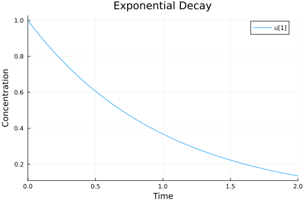

Three variables: The SIR model¶

The SIR model describes the spreading of an contagious disease can be described by the SIR model:

\begin{align} \frac{d}{dt}S(t) &= - \beta S(t)I(t) \\ \frac{d}{dt}I(t) &= \beta S(t)I(t) - \gamma I(t) \\ \frac{d}{dt}R(t) &= \gamma I(t) \end{align}

(2)

State variables

$S(t)$ : the fraction of susceptible people
$I(t)$ : the fraction of infectious people
$R(t)$ : the fraction of recovered (or removed) people

Parameters

$\beta$ : the rate of infection when susceptible and infectious people meet
$\gamma$ : the rate of recovery of infectious people

using OrdinaryDiffEq
using Plots

SIR model (in-place form can save array allocations and thus faster)

function sir!(du, u, p, t)
    s, i, r = u
    β, γ = p
    v1 = β * s * i
    v2 = γ * i
    du[1] = -v1
    du[2] = v1 - v2
    du[3] = v2
    return nothing
end

sir! (generic function with 1 method)

p = (β=1.0, γ=0.3)
u0 = [0.99, 0.01, 0.00]
tspan = (0.0, 20.0)
prob = ODEProblem(sir!, u0, tspan, p)
sol = solve(prob)

retcode: Success
Interpolation: 3rd order Hermite
t: 17-element Vector{Float64}:
  0.0
  0.08921318693905476
  0.3702862715172094
  0.7984257132319627
  1.3237271485666187
  1.991841832691831
  2.7923706947355837
  3.754781614278828
  4.901904318934307
  6.260476636498209
  7.7648912410433075
  9.39040980993922
 11.483861023017885
 13.372369854616487
 15.961357172044833
 18.681426667664056
 20.0
u: 17-element Vector{Vector{Float64}}:
 [0.99, 0.01, 0.0]
 [0.9890894703413342, 0.010634484617786016, 0.00027604504087978485]
 [0.9858331594901347, 0.012901496825852227, 0.0012653436840130792]
 [0.9795270529591532, 0.017282420996456258, 0.003190526044390598]
 [0.9689082167415561, 0.024631267034445452, 0.006460516223998509]
 [0.9490552312363142, 0.03827338797605376, 0.012671380787632129]
 [0.911862947533394, 0.06347250098224955, 0.024664551484356523]
 [0.8398871089274514, 0.11078176031568526, 0.04933113075686341]
 [0.707584206802473, 0.19166147882272797, 0.10075431437479916]
 [0.5081460287219878, 0.2917741934147055, 0.2000797778633069]
 [0.31213222024414106, 0.3415879120018043, 0.34627986775405484]
 [0.1821568309636563, 0.309998313415639, 0.5078448556207048]
 [0.10427205468919257, 0.2206111401113331, 0.6751168051994745]
 [0.07386737407725885, 0.14760143051851196, 0.7785311954042293]
 [0.05545028910907742, 0.07997076922865369, 0.864578941662269]
 [0.04733499069589219, 0.040605653213833574, 0.9120593560902743]
 [0.04522885458929347, 0.02905741611081477, 0.9257137292998918]

Visualize the solution

plot(sol, title="SIR model", xlabel="Time", ylabel="Fraction of population", labels=["S" "I" "R"])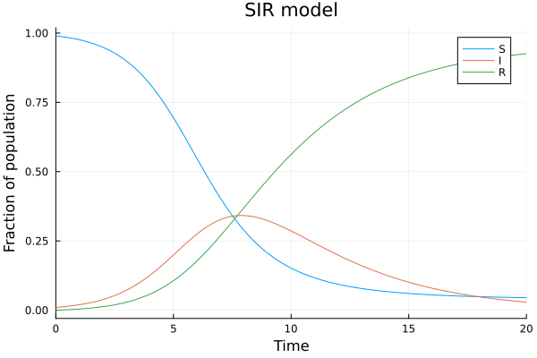

Saving simulation results¶

using DataFrames
using CSV

df = DataFrame(sol)
CSV.write("sir.csv", df)
rm("sir.csv")

This notebook was generated using Literate.jl.