https://
github .com /JuliaPlots /Plots .jl : powerful and convenient visualization with multiple backends. See also Plots.jl docs https://
github .com /JuliaPy /PythonPlot .jl : matplotlibin Julia. See also matplotlib docshttps://
github .com /MakieOrg /Makie .jl : a data visualization ecosystem for the Julia programming language, with high performance and extensibility. See also Makie.jl docs
using PlotsPrepare data then plot
f(x) = sin(sin(x) + 1)
xs = 0.0:0.1:4pi
ys = f.(xs)

plot(xs, ys)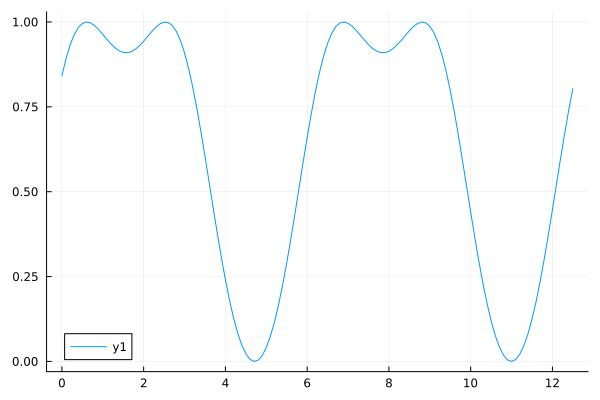
Line plots connect the data points
plot(xs, ys)Scatter plots show the data points only
scatter(xs, ys)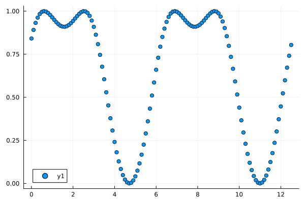
you can trace functions directly
plot(f, xs)Trace a function within a range
plot(f, 0.0, 4pi)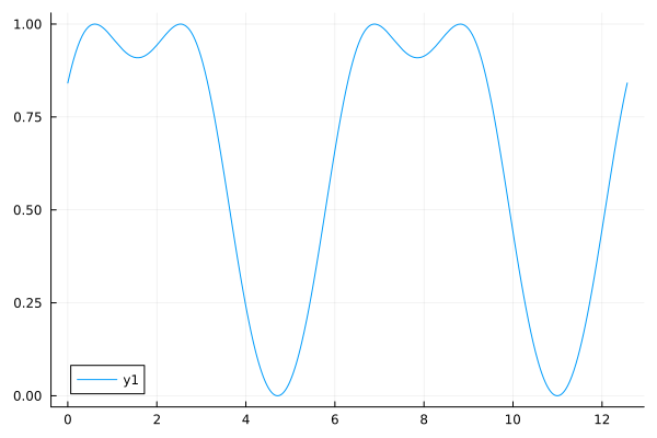
Customization example
plot(f, xs,
    label="My line", legend=:bottom,
    title="My Title",  line=(:red, 3),
    xlim = (0.0, 5.0), ylim = (-1.0, 1.5),
    xlabel="Time", ylabel="My Mood", border=:box)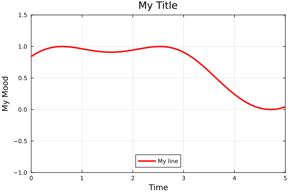
Multiple series: each row is one observation; each column is a variable.
f2(x) = cos(cos(x) + 1)
y2 = f2.(xs)
plot(xs, [ys y2])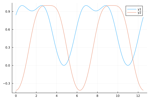
Plotting two functions with customizations
plot(xs, [f, f2], label=["f1" "f2"], linecolor=[:black :green], title="Two time series")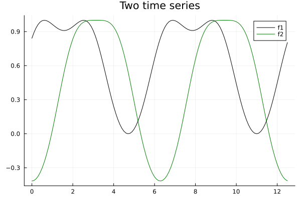
Building the plot in multiple steps in the object-oriented way
xMin = 0.0
xMax = 4.0π
fig = plot(f, xMin, xMax, label="f1", lc=:black)
plot!(fig , f2, xMin, xMax, label="f2", lc=:lightsalmon)
plot!(fig, title = "My title", legend=:outertop)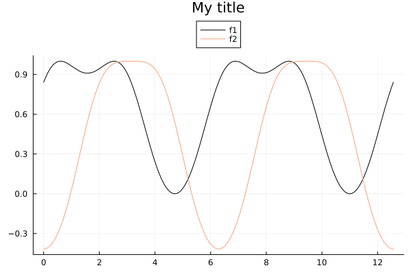
Parametric plot
xₜ(t) = sin(t)
yₜ(t) = sin(2t)

plot(xₜ, yₜ, 0, 2π, leg=false, fill=(0,:orange))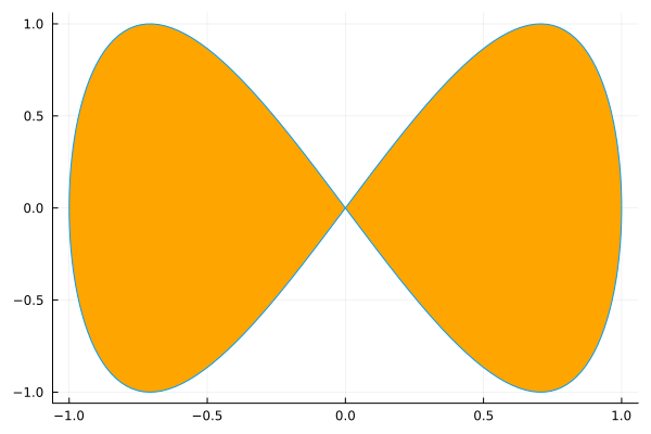
Subplots
ax1 = plot(f, xs)
ax2 = plot(f2, xs)
plot(ax1, ax2)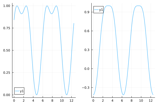
Subplot layout
fig = plot(ax1, ax2, layout=(2, 1))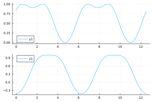
Vector field
Plots.jl
# Quiver plot
quiver(vec(x2d), vec(y2d), quiver=(vec(vx2d), vec(vy2d))

# Or if you have a gradient function ∇f(x,y) -> (vx, vy)
quiver(x2d, y2d, quiver=∇f)
using Plots
using UniformStreamlines∇ = \nabla <TAB>
∇fx = (x, y) -> -y
∇fy = (x, y) -> 1 + x - y^2
#5 (generic function with 1 method)x and y grid points
xs = LinRange(-2, 2, 200)
ys = LinRange(-2, 2, 200)
200-element LinRange{Float64, Int64}:
-2.0, -1.9799, -1.9598, -1.9397, …, 1.9196, 1.9397, 1.9598, 1.9799, 2.0stream object
str = evenstream(xs, ys, ∇fx, ∇fy)StreamlineData{2}: 99 streamlines, 35634 points, domain [-2.0, 2.0] × [-2.0, 2.0]Stream plot
streamlines(str; line_z=colorize(str, :norm), color=:viridis, with_arrows=true, colorbar=false)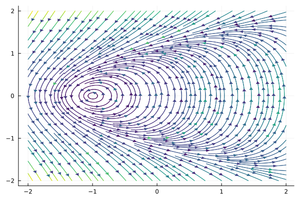
Save figure
savefig([fig_obj,] filename)
Save the current figure
savefig("vector-field.png")"/home/github/actions-runner-2/_work/mmsb-bebi-5009/mmsb-bebi-5009/docs/vector-field.png"Save the figure fig
savefig(fig, "subplots.png")"/home/github/actions-runner-2/_work/mmsb-bebi-5009/mmsb-bebi-5009/docs/subplots.png"This notebook was generated using Literate.jl.