Fig 4.15, 4.16, 4.17

Oscillatory networks.

Figure 4.15 (A)¶

using OrdinaryDiffEq
using ComponentArrays: ComponentArray
using SimpleUnPack
using CairoMakie

function model415(u, p, t)
    @unpack A, B = u
    @unpack k0, k1, k2, n = p
    v1 = k1 * A * (1 + B^n)
    dA = k0 - v1
    dB = v1 - k2 * B
    return (; dA, dB)
end
function model415!(D, u, p, t)
    @unpack dA, dB = model415(u, p, t)
    D.A = dA
    D.B = dB
    nothing
end

model415! (generic function with 1 method)

ps415 = ComponentArray( k0 = 8.0, k1 = 1.0, k2 = 5.0, n = 2.0)
u0415 = ComponentArray( A = 1.5, B = 1.0)
tend = 8.0
prob415 = ODEProblem(model415!, u0415, (0.0, tend), ps415)

ODEProblem with uType ComponentArrays.ComponentVector{Float64, Vector{Float64}, Tuple{ComponentArrays.Axis{(A = 1, B = 2)}}} and tType Float64. In-place: true
Non-trivial mass matrix: false
timespan: (0.0, 8.0)
u0: ComponentVector{Float64}(A = 1.5, B = 1.0)

u0s = [
    ComponentArray(A=1.5, B=1.0),
    ComponentArray(A=0.0, B=1.0),
    ComponentArray(A=0.0, B=3.0),
    ComponentArray(A=2.0, B=0.0),
]

@time sols = map(u0s) do u0
    solve(remake(prob415, u0=u0), Tsit5())
end

fig = Figure()
ax = Axis(fig[1, 1],
    xlabel = "Time",
    ylabel = "Concentration",
    title = "Fig. 4.15 A\nTime series"
)
lines!(ax, 0..tend, t-> sols[1](t).A, label = "A")
lines!(ax, 0..tend, t-> sols[1](t).B, label = "B")
axislegend(ax, position = :rt)
fig

  0.658921 seconds (3.16 M allocations: 213.760 MiB, 8.88% gc time, 99.96% compilation time)

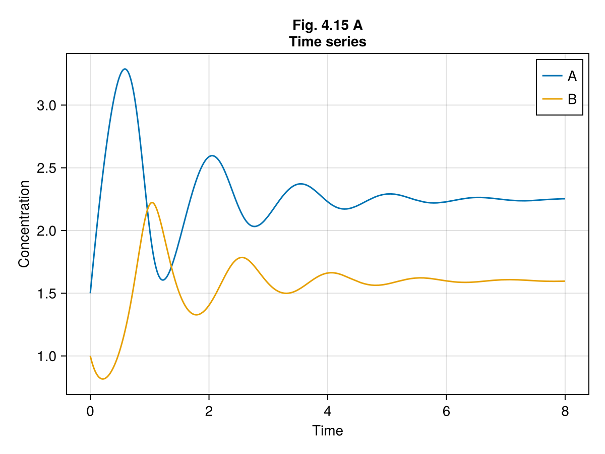
Fig 4.15 (B)¶

∂F415  = function (x, y)
    @unpack dA, dB = model415((; A=x, B=y), ps415, 0.0)
    return Point2d(dA, dB)
end

# Stream plot
fig = Figure(size=(600, 600))
ax = Axis(fig[1, 1],
    xlabel = "[A]",
    ylabel = "[B]",
    title = "Fig. 4.15 B\nPhase plot",
    aspect = 1,
)
streamplot!(ax, ∂F415, 0..4, 0..4)

# Trajectories
for sol in sols
    ts = 0:0.05:tend
    aa = [sol(t).A for t in ts]
    bb = [sol(t).B for t in ts]
    lines!(ax, aa, bb)
end
limits!(ax, 0.0, 4.0, 0.0, 4.0)

# Nullclines
xx = 0:0.01:4
yy = 0:0.01:4
∂A415 = [model415((; A=x, B=y), ps415, nothing).dA for x in xx, y in yy]
∂B415 = [model415((; A=x, B=y), ps415, nothing).dB for x in xx, y in yy]
contour!(ax, xx, yy, ∂A415, levels=[0], color=:black, linestyle=:solid, linewidth=2, label="A nullcline")
contour!(ax, xx, yy, ∂B415, levels=[0], color=:black, linestyle=:dash, linewidth=2, label="B nullcline")
axislegend(ax, position = :rb)
fig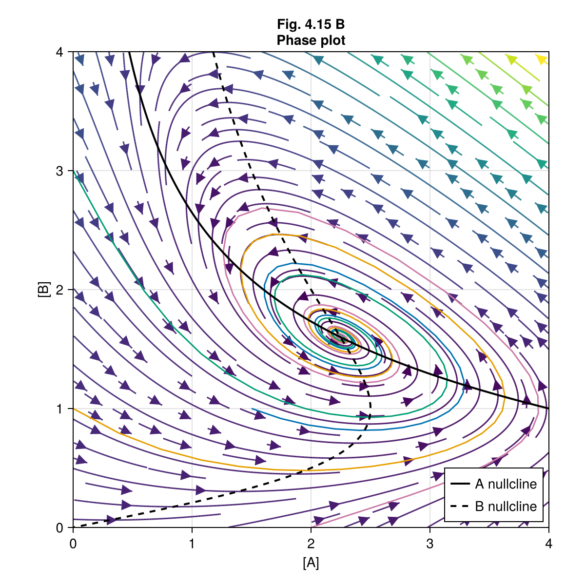

Fig 4.16 A¶

Oscillatory parameter set

ps416 = ComponentArray( k0 = 8.0, k1 = 1.0, k2 = 5.0, n = 2.5)
tend = 100.0
u0s = [
    ComponentArray(A=1.5, B=1.0),
    ComponentArray(A=0.0, B=1.0),
    ComponentArray(A=0.0, B=3.0),
    ComponentArray(A=2.0, B=0.0),
]

prob416 = ODEProblem(model415!, u0415, tend, ps416)
@time sols = map(u0s) do u0
    solve(remake(prob416, u0=u0), Tsit5())
end

fig = Figure()
ax = Axis(fig[1, 1],
    xlabel = "Time",
    ylabel = "Concentration",
    title = "Fig. 4.16 A\nTime series"
)
lines!(ax, 0..8, t-> sols[1](t).A, label = "A")
lines!(ax, 0..8, t-> sols[1](t).B, label = "B")
axislegend(ax, position = :rt)
fig

  0.030110 seconds (45.60 k allocations: 3.243 MiB, 96.95% compilation time)

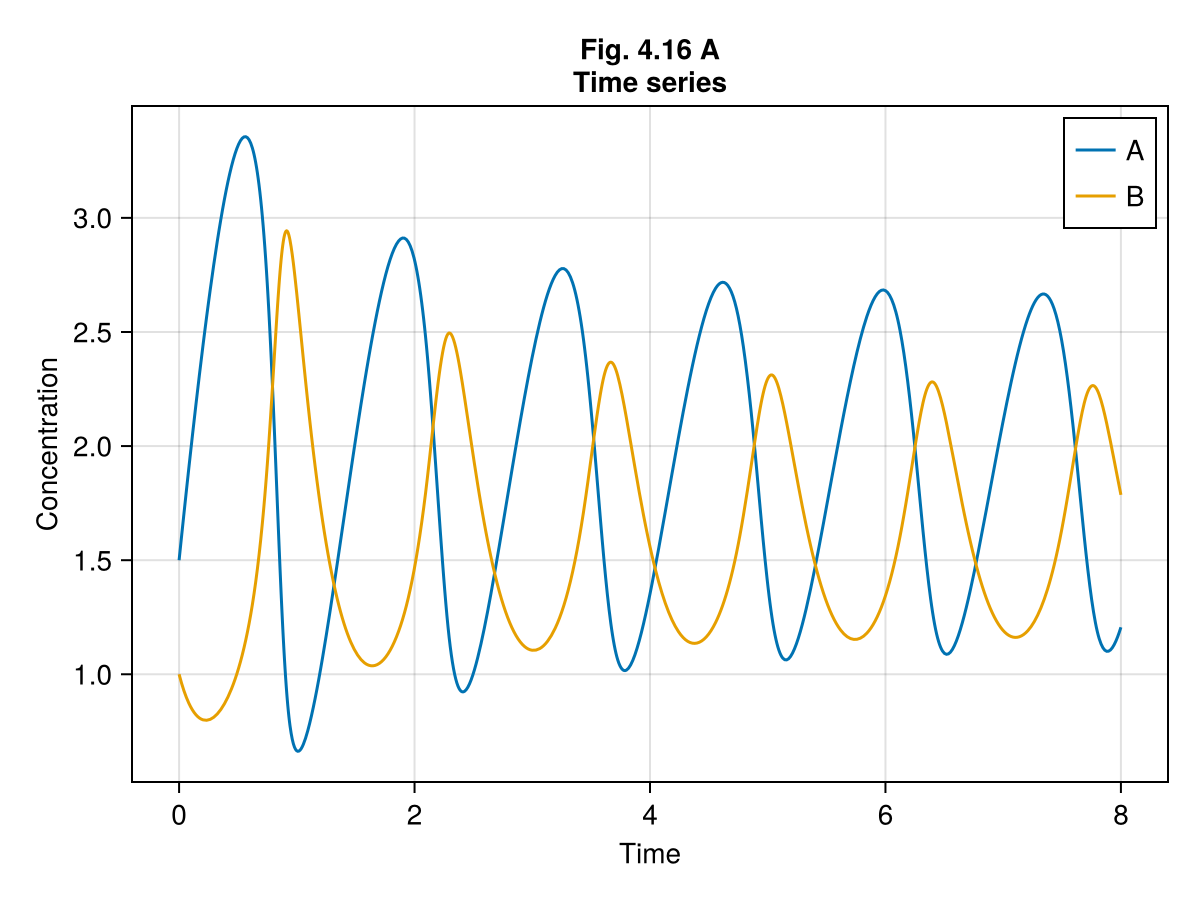
Fig 4.16 b¶

∂F416 = function (x, y)
    @unpack dA, dB = model415((; A=x, B=y), ps416, nothing)
    return Point2d(dA, dB)
end

fig = Figure(size=(600, 600))
ax = Axis(fig[1, 1],
    xlabel = "[A]",
    ylabel = "[B]",
    title = "Fig. 4.16 B\nPhase plot",
    aspect = 1,
)

# Stream plot
streamplot!(ax, ∂F416, 0..4, 0..4)

# Nullclines
xx = 0:0.01:4
yy = 0:0.01:4
∂A416 = [model415((; A=x, B=y), ps416, nothing).dA for x in xx, y in yy]
∂B416 = [model415((; A=x, B=y), ps416, nothing).dB for x in xx, y in yy]

contour!(ax, xx, yy, ∂A416, levels=[0], color=:black, linestyle=:solid, linewidth=2, label="A nullcline")
contour!(ax, xx, yy, ∂B416, levels=[0], color=:black, linestyle=:dash, linewidth=2, label="B nullcline")

# Trajectories
for sol in sols
    ts = 0:0.01:tend
    aa = [sol(t).A for t in ts]
    bb = [sol(t).B for t in ts]
    lines!(ax, aa, bb, color=:tomato)
end
axislegend(ax, position = :rc)
limits!(ax, 0.0, 4.0, 0.0, 4.0)
fig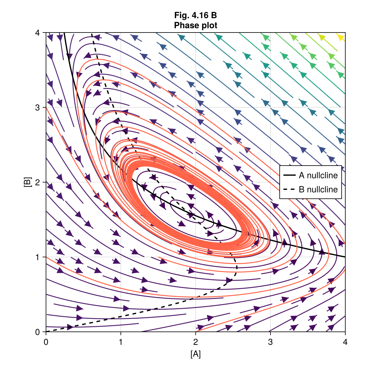

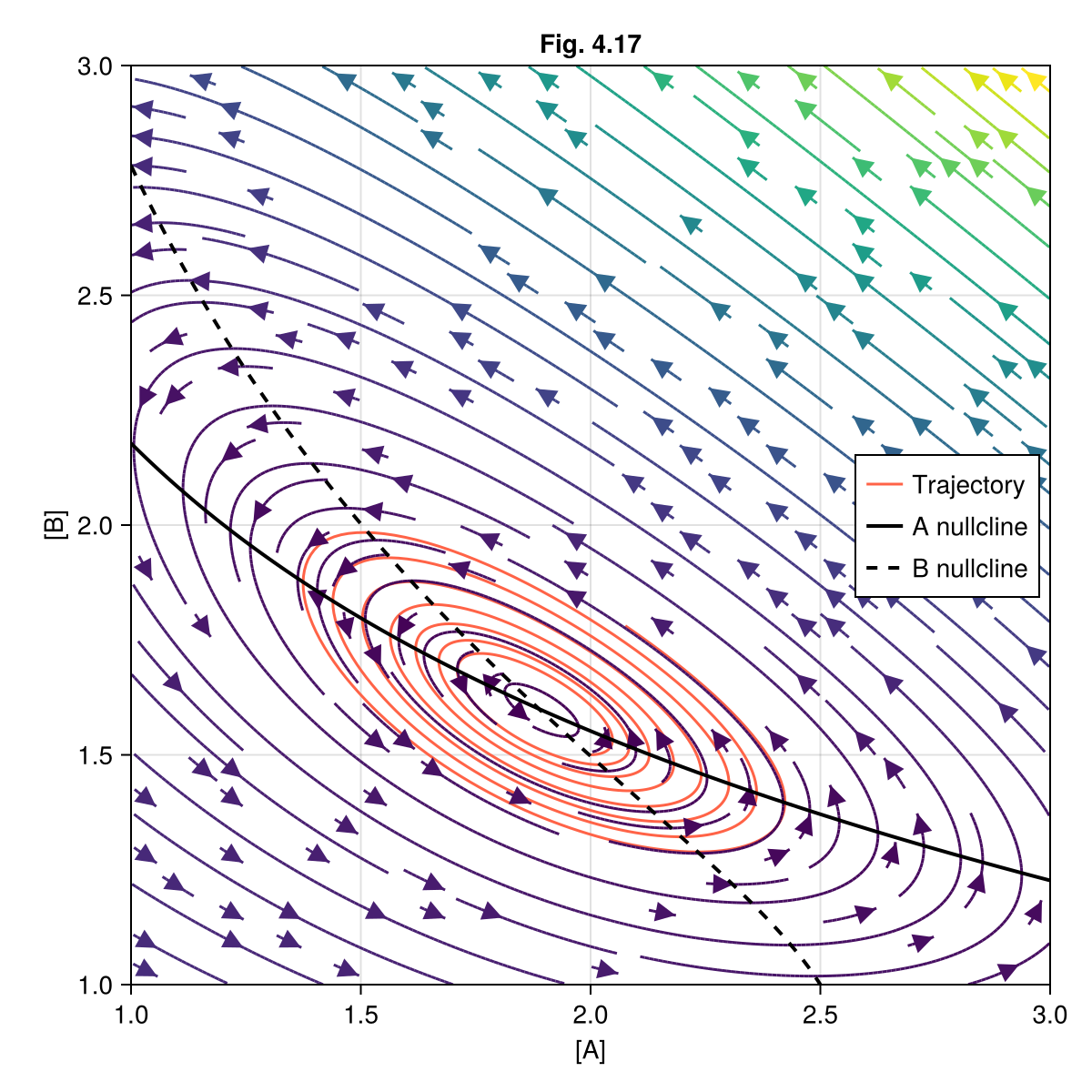
Fig 4.17¶

prob417 = remake(prob415, p=ps416, u0=ComponentArray(A=2.0, B=1.5), tspan=(0.0, 10.0))
@time sol = solve(prob417, Tsit5())

fig = Figure(size=(600, 600))
ax = Axis(fig[1, 1],
    xlabel = "[A]",
    ylabel = "[B]",
    title = "Fig. 4.17",
    aspect = 1,
)

lines!(ax, sol, idxs=(1, 2), color=:tomato, label="Trajectory")
xx = 1:0.01:3
yy = 1:0.01:3
∂A417 = [model415((; A=x, B=y), ps416, nothing).dA for x in xx, y in yy]
∂B417 = [model415((; A=x, B=y), ps416, nothing).dB for x in xx, y in yy];

streamplot!(ax, ∂F416, xx, yy)
contour!(ax, xx, yy, ∂A417, levels=[0], color=:black, linestyle=:solid, linewidth=2, label="A nullcline")
contour!(ax, xx, yy, ∂B417, levels=[0], color=:black, linestyle=:dash, linewidth=2, label="B nullcline")
axislegend(ax, position = :rc)
limits!(ax, 1.0, 3.0, 1.0, 3.0)
fig

  0.000034 seconds (422 allocations: 33.227 KiB)

This notebook was generated using Literate.jl.