Fig 2.11, 2.12, 2.13, 2.14

Model reduction of ODE metabolic networks.

using OrdinaryDiffEq
using ComponentArrays: ComponentArray
using SimpleUnPack
using CairoMakie

function model211!(du, u, p, t)
    @unpack k0, k1, km1, k2 = p
    @unpack A, B = u
    v0 = k0
    v1 = k1 * A - km1 * B
    v2 = k2 * B
    du.A = v0 - v1
    du.B = v1 - v2
    nothing
end

model211! (generic function with 1 method)

ps211 = ComponentArray(k0=0.0, k1=9.0, km1=12.0, k2=2.0)
u0 = ComponentArray(A=0.0, B=10.0)
tend = 3.0
prob211 = ODEProblem(model211!, u0, tend, ps211)

ODEProblem with uType ComponentArrays.ComponentVector{Float64, Vector{Float64}, Tuple{ComponentArrays.Axis{(A = 1, B = 2)}}} and tType Float64. In-place: true
Non-trivial mass matrix: false
timespan: (0.0, 3.0)
u0: ComponentVector{Float64}(A = 0.0, B = 10.0)

@time sol211 = solve(prob211, Tsit5())

  0.985928 seconds (4.85 M allocations: 323.347 MiB, 8.64% gc time, 100.00% compilation time)

retcode: Success
Interpolation: specialized 4th order "free" interpolation
t: 35-element Vector{Float64}:
 0.0
 8.33250002662905e-6
 9.165750029291953e-5
 0.0009249075029558242
 0.0049255520098868185
 0.012950994848397006
 0.0242033909176605
 0.0386770307390286
 0.056874831424329884
 0.0788503957456076
 ⋮
 1.8976419863766623
 2.04653471747305
 2.199447644522893
 2.3553401128119527
 2.512411490644732
 2.6691958789164265
 2.8250502965479143
 2.9800392317414297
 3.0
u: 35-element Vector{ComponentArrays.ComponentVector{Float64, Vector{Float64}, Tuple{ComponentArrays.Axis{(A = 1, B = 2)}}}}:
 ComponentVector{Float64}(A = 0.0, B = 10.0)
 ComponentVector{Float64}(A = 0.0009998041949395534, B = 9.99883355552422)
 ComponentVector{Float64}(A = 0.010987314386434823, B = 9.987180710981443)
 ComponentVector{Float64}(A = 0.10981641889273347, B = 9.871804396920822)
 ComponentVector{Float64}(A = 0.5587746014145984, B = 9.345993049721082)
 ComponentVector{Float64}(A = 1.3433471992221448, B = 8.419063000156342)
 ComponentVector{Float64}(A = 2.2233611282304873, B = 7.361953780480142)
 ComponentVector{Float64}(A = 3.0603231048671335, B = 6.327621136104826)
 ComponentVector{Float64}(A = 3.7711572231276924, B = 5.4043546428642255)
 ComponentVector{Float64}(A = 4.28969045038158, B = 4.665729178966638)
 ⋮
 ComponentVector{Float64}(A = 1.2038103571647432, B = 0.822017536833704)
 ComponentVector{Float64}(A = 1.0669057534967417, B = 0.7284268312399474)
 ComponentVector{Float64}(A = 0.9424542249340166, B = 0.6434317390046304)
 ComponentVector{Float64}(A = 0.8304907306491801, B = 0.5670029920694248)
 ComponentVector{Float64}(A = 0.7311216458221879, B = 0.4991830768257472)
 ComponentVector{Float64}(A = 0.6437926931468013, B = 0.43957679348536416)
 ComponentVector{Float64}(A = 0.567326932045669, B = 0.3873753245348317)
 ComponentVector{Float64}(A = 0.5002984513219507, B = 0.3416083359534354)
 ComponentVector{Float64}(A = 0.49230199214988013, B = 0.3360780170065645)

Fig 2.11

ts = range(0, tend, length=100)
us = Array(sol211(ts))
fig, ax, sp = series(ts, us, labels=["A", "B"], axis=(xlabel="Time", ylabel="Concentration", title="Fig 2.11\nFull model"))
axislegend(ax, position=:rt)
fig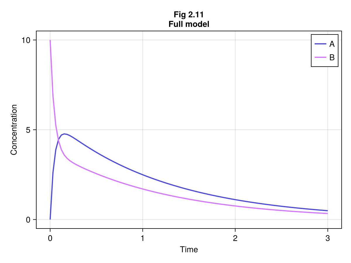

Figure 2.12¶

Rapid equilibrium assumption

function model212(u, p, t)
    @unpack k0, k1, km1, k2 = p
    @unpack C = u
    A = C * km1 / (km1 + k1)
    B = C * k1 / (km1 + k1)
    return (; A, B, dC = k0 - k2 * B)
end
function model212!(du, u, p, t)
    @unpack dC = model212(u, p, t)
    du.C = dC
    nothing
end

model212! (generic function with 1 method)

tend = 3.0
u0212 = ComponentArray(C=10.0)
prob212 = ODEProblem(model212!, u0212, tend, ps211)

ODEProblem with uType ComponentArrays.ComponentVector{Float64, Vector{Float64}, Tuple{ComponentArrays.Axis{(C = 1,)}}} and tType Float64. In-place: true
Non-trivial mass matrix: false
timespan: (0.0, 3.0)
u0: ComponentVector{Float64}(C = 10.0)

@time sol212 = solve(prob212, Tsit5())

  0.786822 seconds (4.62 M allocations: 307.734 MiB, 9.04% gc time, 100.00% compilation time)

retcode: Success
Interpolation: specialized 4th order "free" interpolation
t: 9-element Vector{Float64}:
 0.0
 0.10313309318586757
 0.3753972361702897
 0.7370512456211995
 1.167737125797318
 1.6758020636903974
 2.2474174188288836
 2.8795734914073643
 3.0
u: 9-element Vector{ComponentArrays.ComponentVector{Float64, Vector{Float64}, Tuple{ComponentArrays.Axis{(C = 1,)}}}}:
 ComponentVector{Float64}(C = 10.0)
 ComponentVector{Float64}(C = 9.153948340781719)
 ComponentVector{Float64}(C = 7.24865584846079)
 ComponentVector{Float64}(C = 5.3165629074890655)
 ComponentVector{Float64}(C = 3.6754225790588735)
 ComponentVector{Float64}(C = 2.377822615503587)
 ComponentVector{Float64}(C = 1.4567854018333606)
 ComponentVector{Float64}(C = 0.8473770113337572)
 ComponentVector{Float64}(C = 0.7642714199479234)

fig = Figure()
ax = Axis(
    fig[1, 1],
    xlabel="Time",
    ylabel="Concentration",
    title="Fig. 2.12\nRapid equilibrium model"
)

lines!(ax, 0 .. tend, t -> sol211(t).A, label="A (full solution)", linestyle=:dash)
lines!(ax, 0 .. tend, t -> sol211(t).B, label="B (full solution)", linestyle=:dash)
lines!(ax, 0 .. tend, t -> model212(sol212(t), ps211, t).A, label="A (rapid equilibrium)")
lines!(ax, 0 .. tend, t -> model212(sol212(t), ps211, t).B, label="B (rapid equilibrium)")
axislegend(ax, position=:rt)
fig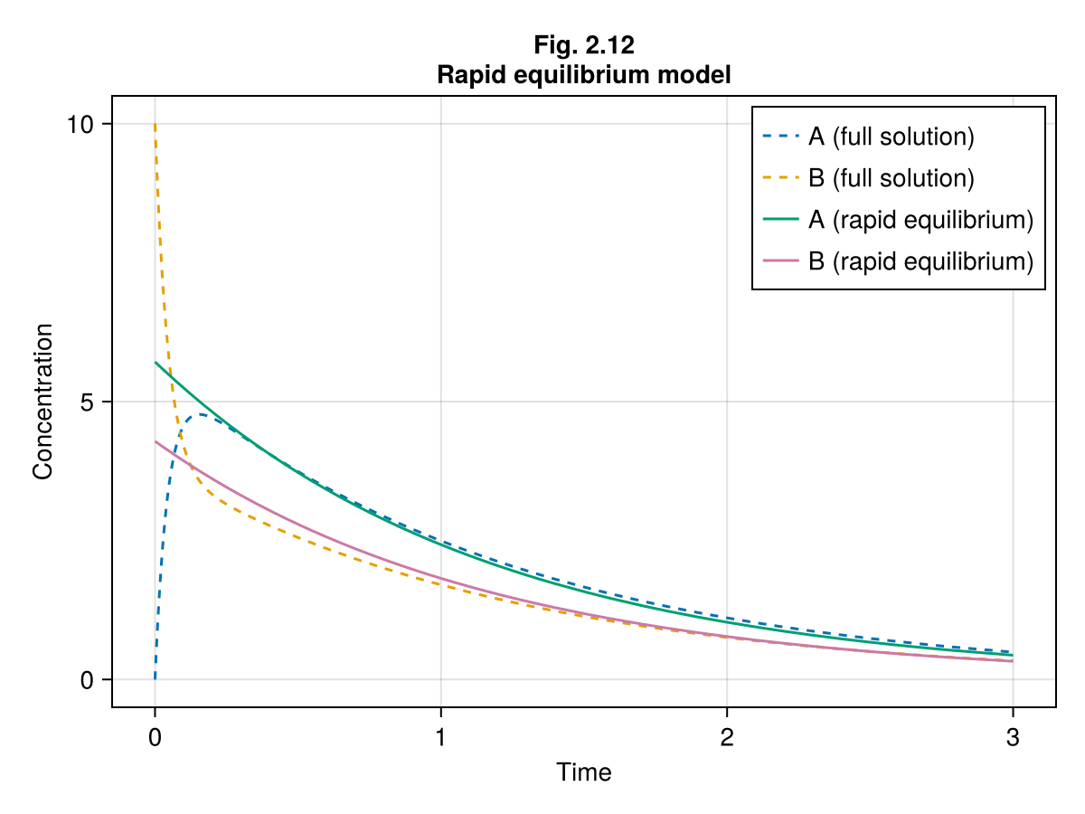

Figure 2.13¶

Rapid equilibrium (take 2) When another set of parameters is not suitable for rapid equilibrium assumption.

ps213 = ComponentArray(k0=9.0, k1=20.0, km1=12.0, k2=2.0)
u0 = ComponentArray(A=8.0, B=4.0)
tend = 3.0

@time sol213full = solve(ODEProblem(model211!, u0, tend, ps213), Tsit5())
@time sol213re = solve(ODEProblem(model212!, ComponentArray(C=sum(u0)), tend, ps213), Tsit5())

  0.000079 seconds (444 allocations: 32.555 KiB)
  0.013487 seconds (23.89 k allocations: 1.606 MiB, 99.14% compilation time)

retcode: Success
Interpolation: specialized 4th order "free" interpolation
t: 9-element Vector{Float64}:
 0.0
 0.10985788520382275
 0.3514885215968111
 0.6586777912438853
 1.0393785582716237
 1.4959514209075846
 2.0369831593840857
 2.672183436982096
 3.0
u: 9-element Vector{ComponentArrays.ComponentVector{Float64, Vector{Float64}, Tuple{ComponentArrays.Axis{(C = 1,)}}}}:
 ComponentVector{Float64}(C = 12.0)
 ComponentVector{Float64}(C = 11.384108095813616)
 ComponentVector{Float64}(C = 10.293352240189927)
 ComponentVector{Float64}(C = 9.307008837373226)
 ComponentVector{Float64}(C = 8.509173268418104)
 ComponentVector{Float64}(C = 7.939847552423305)
 ComponentVector{Float64}(C = 7.576224445585626)
 ComponentVector{Float64}(C = 7.370083403215763)
 ComponentVector{Float64}(C = 7.312901875215382)

fig = Figure()
ax = Axis(
    fig[1, 1],
    xlabel="Time",
    ylabel="Concentration",
    title="Fig. 2.13\nFull vs Rapid equilibrium"
)
lines!(ax, 0 .. tend, t -> sol213full(t).A, label="A (full solution)", linestyle=:dash)
lines!(ax, 0 .. tend, t -> sol213full(t).B, label="B (full solution)", linestyle=:dash)
lines!(ax, 0 .. tend, t -> model212(sol213re(t), ps213, t).A, label="A (rapid equilibrium)")
lines!(ax, 0 .. tend, t -> model212(sol213re(t), ps213, t).B, label="B (rapid equilibrium)")
axislegend(ax, position=:rt)
fig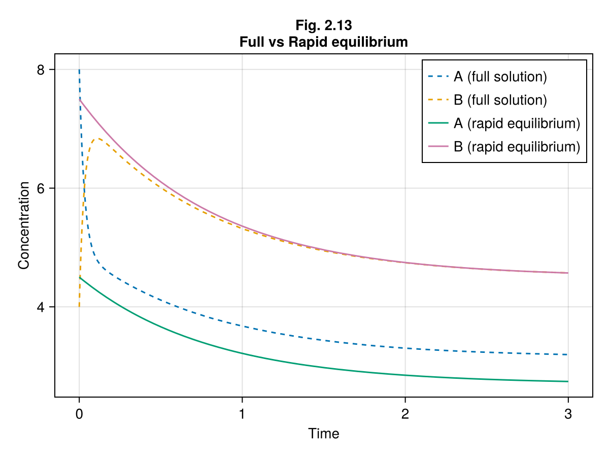

Figure 2.14 : QSSA¶

Quasi-steady state assumption on species A

_a214(u, p, t) = (p.k0 + p.km1 * u.B) / p.k1
_u0214(u0, p) = (p.k1 * u0 - p.k0) / (p.k1 + p.km1)
function model214!(du, u, p, t)
    @unpack k0, k1, km1, k2 = p
    @unpack B = u
    A = _a214(u, p, t)
    du.B = k1 * A - (km1 + k2) * B
    nothing
end

ps214 = ps213
u0214 = ComponentArray(B=_u0214(sum(u0), ps214))

ComponentVector{Float64}(B = 7.21875)

Solve QSSA model

@time sol214 = solve(ODEProblem(model214!, u0214, tend, ps214), Tsit5())

  0.819424 seconds (4.69 M allocations: 312.510 MiB, 11.37% gc time, 99.95% compilation time)

retcode: Success
Interpolation: specialized 4th order "free" interpolation
t: 11-element Vector{Float64}:
 0.0
 0.09213371408627126
 0.25808536714860464
 0.457920051925288
 0.7105343436489328
 1.0087389301910419
 1.3646427389483302
 1.7813284300909857
 2.2736032336012837
 2.8565647706624135
 3.0
u: 11-element Vector{ComponentArrays.ComponentVector{Float64, Vector{Float64}, Tuple{ComponentArrays.Axis{(B = 1,)}}}}:
 ComponentVector{Float64}(B = 7.21875)
 ComponentVector{Float64}(B = 6.7612206800899255)
 ComponentVector{Float64}(B = 6.12255437765173)
 ComponentVector{Float64}(B = 5.587991174239103)
 ComponentVector{Float64}(B = 5.156461156294923)
 ComponentVector{Float64}(B = 4.861574058275949)
 ComponentVector{Float64}(B = 4.677452877572093)
 ComponentVector{Float64}(B = 4.577129236517502)
 ComponentVector{Float64}(B = 4.528831303746667)
 ComponentVector{Float64}(B = 4.509002572522133)
 ComponentVector{Float64}(B = 4.50675741206795)

fig = Figure()
ax = Axis(
    fig[1, 1],
    xlabel="Time",
    ylabel="Concentration",
    title="Fig. 2.14\nQSSA vs Full model"
)
lines!(ax, 0 .. tend, t -> sol213full(t).A, label="A (full solution)", linestyle=:dash)
lines!(ax, 0 .. tend, t -> sol213full(t).B, label="B (full solution)", linestyle=:dash)
lines!(ax, 0 .. tend, t -> _a214(sol214(t), ps214, t), label="A (QSSA)")
lines!(ax, 0 .. tend, t -> sol214(t).B, label="B (QSSA)")
axislegend(ax, position=:rt)
fig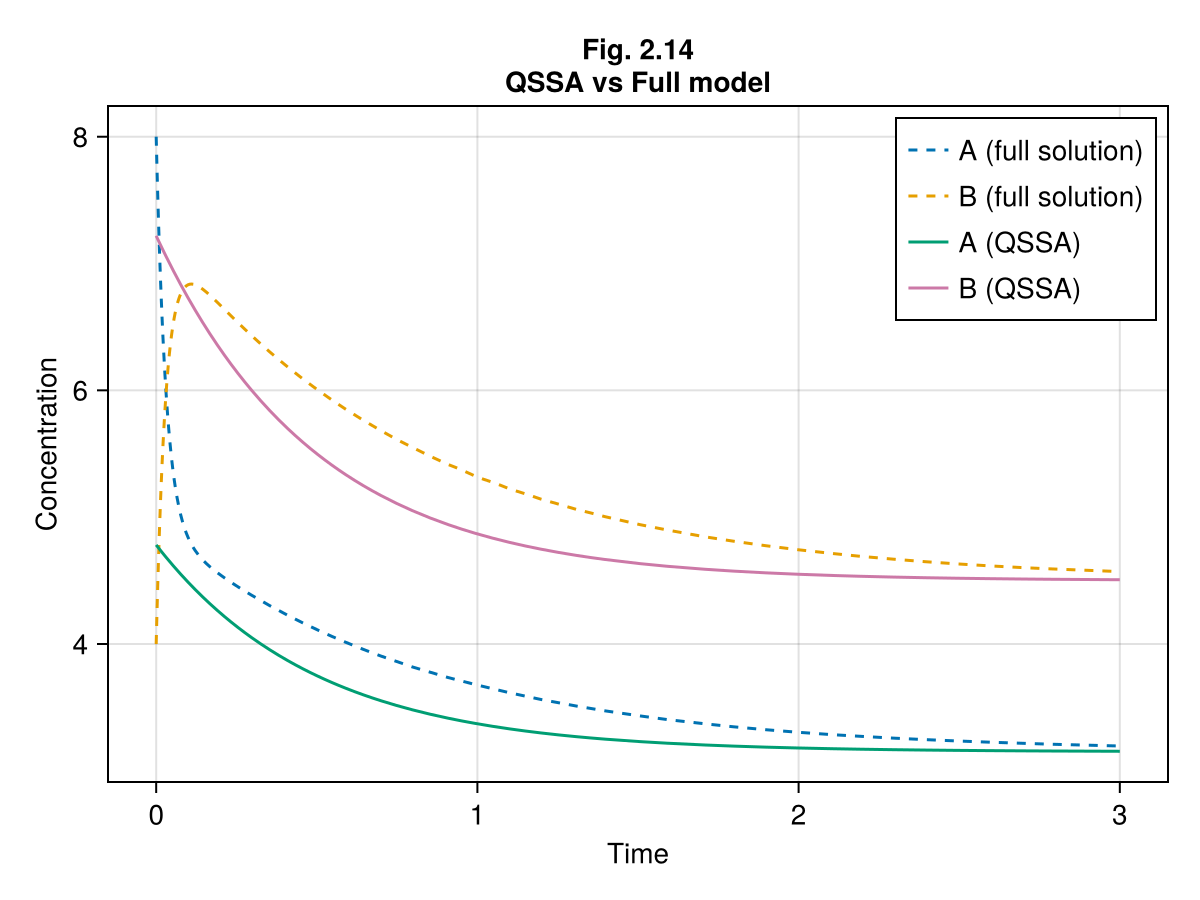

This notebook was generated using Literate.jl.